Electronegativity#
- Page ID
- 9369
\( \newcommand{\vecs}[1]{\overset { \scriptstyle \rightharpoonup} {\mathbf{#1}} } \)
\( \newcommand{\vecd}[1]{\overset{-\!-\!\rightharpoonup}{\vphantom{a}\smash {#1}}} \)
\( \newcommand{\id}{\mathrm{id}}\) \( \newcommand{\Span}{\mathrm{span}}\)
( \newcommand{\kernel}{\mathrm{null}\,}\) \( \newcommand{\range}{\mathrm{range}\,}\)
\( \newcommand{\RealPart}{\mathrm{Re}}\) \( \newcommand{\ImaginaryPart}{\mathrm{Im}}\)
\( \newcommand{\Argument}{\mathrm{Arg}}\) \( \newcommand{\norm}[1]{\| #1 \|}\)
\( \newcommand{\inner}[2]{\langle #1, #2 \rangle}\)
\( \newcommand{\Span}{\mathrm{span}}\)
\( \newcommand{\id}{\mathrm{id}}\)
\( \newcommand{\Span}{\mathrm{span}}\)
\( \newcommand{\kernel}{\mathrm{null}\,}\)
\( \newcommand{\range}{\mathrm{range}\,}\)
\( \newcommand{\RealPart}{\mathrm{Re}}\)
\( \newcommand{\ImaginaryPart}{\mathrm{Im}}\)
\( \newcommand{\Argument}{\mathrm{Arg}}\)
\( \newcommand{\norm}[1]{\| #1 \|}\)
\( \newcommand{\inner}[2]{\langle #1, #2 \rangle}\)
\( \newcommand{\Span}{\mathrm{span}}\) \( \newcommand{\AA}{\unicode[.8,0]{x212B}}\)
\( \newcommand{\vectorA}[1]{\vec{#1}} % arrow\)
\( \newcommand{\vectorAt}[1]{\vec{\text{#1}}} % arrow\)
\( \newcommand{\vectorB}[1]{\overset { \scriptstyle \rightharpoonup} {\mathbf{#1}} } \)
\( \newcommand{\vectorC}[1]{\textbf{#1}} \)
\( \newcommand{\vectorD}[1]{\overrightarrow{#1}} \)
\( \newcommand{\vectorDt}[1]{\overrightarrow{\text{#1}}} \)
\( \newcommand{\vectE}[1]{\overset{-\!-\!\rightharpoonup}{\vphantom{a}\smash{\mathbf {#1}}}} \)
\( \newcommand{\vecs}[1]{\overset { \scriptstyle \rightharpoonup} {\mathbf{#1}} } \)
\( \newcommand{\vecd}[1]{\overset{-\!-\!\rightharpoonup}{\vphantom{a}\smash {#1}}} \)
\(\newcommand{\avec}{\mathbf a}\) \(\newcommand{\bvec}{\mathbf b}\) \(\newcommand{\cvec}{\mathbf c}\) \(\newcommand{\dvec}{\mathbf d}\) \(\newcommand{\dtil}{\widetilde{\mathbf d}}\) \(\newcommand{\evec}{\mathbf e}\) \(\newcommand{\fvec}{\mathbf f}\) \(\newcommand{\nvec}{\mathbf n}\) \(\newcommand{\pvec}{\mathbf p}\) \(\newcommand{\qvec}{\mathbf q}\) \(\newcommand{\svec}{\mathbf s}\) \(\newcommand{\tvec}{\mathbf t}\) \(\newcommand{\uvec}{\mathbf u}\) \(\newcommand{\vvec}{\mathbf v}\) \(\newcommand{\wvec}{\mathbf w}\) \(\newcommand{\xvec}{\mathbf x}\) \(\newcommand{\yvec}{\mathbf y}\) \(\newcommand{\zvec}{\mathbf z}\) \(\newcommand{\rvec}{\mathbf r}\) \(\newcommand{\mvec}{\mathbf m}\) \(\newcommand{\zerovec}{\mathbf 0}\) \(\newcommand{\onevec}{\mathbf 1}\) \(\newcommand{\real}{\mathbb R}\) \(\newcommand{\twovec}[2]{\left[\begin{array}{r}#1 \\ #2 \end{array}\right]}\) \(\newcommand{\ctwovec}[2]{\left[\begin{array}{c}#1 \\ #2 \end{array}\right]}\) \(\newcommand{\threevec}[3]{\left[\begin{array}{r}#1 \\ #2 \\ #3 \end{array}\right]}\) \(\newcommand{\cthreevec}[3]{\left[\begin{array}{c}#1 \\ #2 \\ #3 \end{array}\right]}\) \(\newcommand{\fourvec}[4]{\left[\begin{array}{r}#1 \\ #2 \\ #3 \\ #4 \end{array}\right]}\) \(\newcommand{\cfourvec}[4]{\left[\begin{array}{c}#1 \\ #2 \\ #3 \\ #4 \end{array}\right]}\) \(\newcommand{\fivevec}[5]{\left[\begin{array}{r}#1 \\ #2 \\ #3 \\ #4 \\ #5 \\ \end{array}\right]}\) \(\newcommand{\cfivevec}[5]{\left[\begin{array}{c}#1 \\ #2 \\ #3 \\ #4 \\ #5 \\ \end{array}\right]}\) \(\newcommand{\mattwo}[4]{\left[\begin{array}{rr}#1 \amp #2 \\ #3 \amp #4 \\ \end{array}\right]}\) \(\newcommand{\laspan}[1]{\text{Span}\{#1\}}\) \(\newcommand{\bcal}{\cal B}\) \(\newcommand{\ccal}{\cal C}\) \(\newcommand{\scal}{\cal S}\) \(\newcommand{\wcal}{\cal W}\) \(\newcommand{\ecal}{\cal E}\) \(\newcommand{\coords}[2]{\left\{#1\right\}_{#2}}\) \(\newcommand{\gray}[1]{\color{gray}{#1}}\) \(\newcommand{\lgray}[1]{\color{lightgray}{#1}}\) \(\newcommand{\rank}{\operatorname{rank}}\) \(\newcommand{\row}{\text{Row}}\) \(\newcommand{\col}{\text{Col}}\) \(\renewcommand{\row}{\text{Row}}\) \(\newcommand{\nul}{\text{Nul}}\) \(\newcommand{\var}{\text{Var}}\) \(\newcommand{\corr}{\text{corr}}\) \(\newcommand{\len}[1]{\left|#1\right|}\) \(\newcommand{\bbar}{\overline{\bvec}}\) \(\newcommand{\bhat}{\widehat{\bvec}}\) \(\newcommand{\bperp}{\bvec^\perp}\) \(\newcommand{\xhat}{\widehat{\xvec}}\) \(\newcommand{\vhat}{\widehat{\vvec}}\) \(\newcommand{\uhat}{\widehat{\uvec}}\) \(\newcommand{\what}{\widehat{\wvec}}\) \(\newcommand{\Sighat}{\widehat{\Sigma}}\) \(\newcommand{\lt}{<}\) \(\newcommand{\gt}{>}\) \(\newcommand{\amp}{&}\) \(\definecolor{fillinmathshade}{gray}{0.9}\)Electronegativity
Molecules are collections of atoms that are associated with one another through bonds. It is reasonable to expect—and the case empirically—that different atoms will exhibit different physical properties, including abilities to interact with other atoms. One such property, the tendency of an atom to attract electrons, is described by the chemical concept and term, electronegativity. While several methods for measuring electronegativity have been developed, the one most commonly taught to biologists is the one created by Linus Pauling.
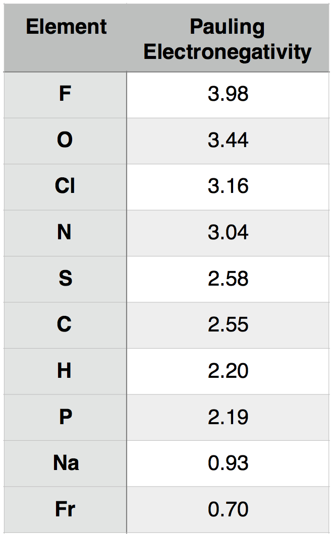
A description of how Pauling electronegativity can be calculated is beyond the scope of BIS2A. What is important to know, however, is that electronegativity values have been experimentally and/or theoretically determined for nearly all elements in the periodic table. The values are unitless and are reported relative to the standard reference, hydrogen, whose electronegativity is 2.20. The larger the electronegativity value, the greater tendency an atom has to attract electrons. Using this scale, the electronegativity of different atoms can be quantitatively compared. For instance, by using Table 1 below, you could report that oxygen atoms are more electronegative than phosphorous atoms.

Table 1. Pauling electronegativity values for select elements of relevance to BIS2A as well as elements at the two extremes (highest and lowest) of the electronegativity scale.
Attribution: Marc T. Facciotti (original work)
The utility of the Pauling electronegativity scale in BIS2A is to provide a chemical basis for explaining the types of bonds that form between the commonly occurring elements in biological systems and to explain some of the key interactions that we observe routinely. We develop our understanding of electronegativity-based arguments about bonds and molecular interactions by comparing the electronegativities of two atoms. Recall, the larger the electronegativity, the stronger the "pull" an atom exerts on nearby electrons.
We can consider, for example, the common interaction between oxygen (O) and hydrogen (H). Let us assume that O and H are interacting (forming a bond) and write that interaction as O-H, where the dash between the letters represents the interaction between the two atoms. To understand this interaction better, we can compare the relative electronegativity of each atom. Examining the table above, we see that O has an electronegativity of 3.44, and H has an electronegativity of 2.20.
Based on the concept of electronegativity as we now understand it, we can surmise that the oxygen (O) atom will tend to "pull" the electrons away from the hydrogen (H) when they are interacting. This will give rise to a slight but significant negative charge around the O atom (due to the higher tendency of the electrons to be associated with the O atom). This also results in a slight positive charge around the H atom (due to the decrease in the probability of finding an electron nearby). Since the electrons are not distributed evenly between the two atoms AND, by consequence, the electric charge is also not evenly distributed, we describe this interaction or bond as polar. There are two poles in effect: the negative pole near the oxygen and the positive pole near the hydrogen.
To extend the utility of this concept, we can now ask how an interaction between oxygen (O) and hydrogen (H) differs from an interaction between sulfur (S) and hydrogen (H). That is, how does O-H differ from S-H? If we examine the table above, we see that the difference in electronegativity between O and H is 1.24 (3.44 - 2.20 = 1.24) and that the difference in electronegativity between S and H is 0.38 (2.58 – 2.20 = 0.38). We can therefore conclude that an O-H bond is more polar than an S-H bond. We will discuss the consequences of these differences in subsequent chapters.

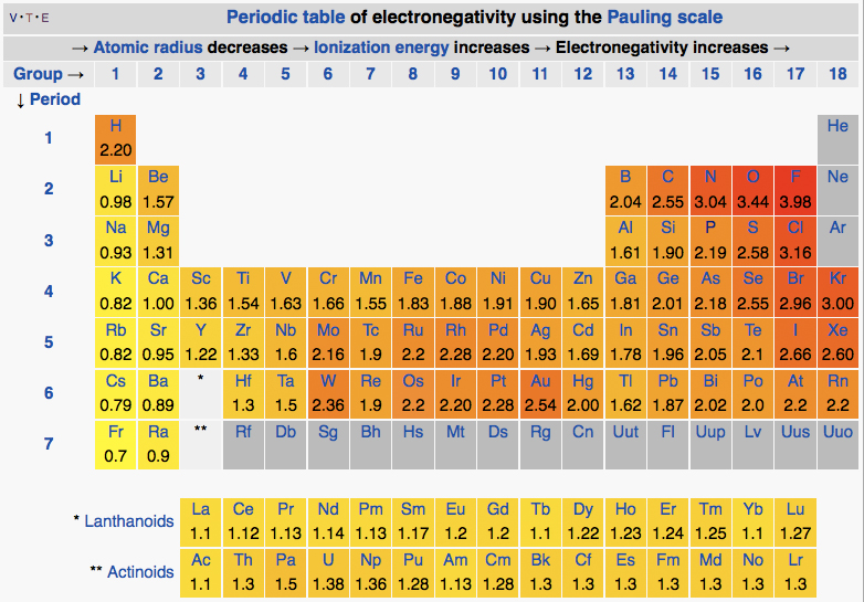
Figure 2. The periodic table with the electronegativities of each atom listed.
Attribution: By DMacks (https://en.wikipedia.org/wiki/Electronegativity) [CC BY-SA 3.0 (http://creativecommons.org/licenses/by-sa/3.0)], via Wikimedia Commons
An examination of the periodic table of the elements (Figure 2) illustrates that electronegativity is related to some of the physical properties used to organize the elements into the table. Certain trends are apparent. For instance, those atoms with the largest electronegativity tend to reside in the upper right hand corner of the periodic table, such as Fluorine (F), Oxygen (O) and Chlorine (Cl), while elements with the smallest electronegativity tend to be found at the other end of the table, in the lower left, such as Francium (Fr), Cesium (Cs) and Radium (Ra).
More information on electronegativity can be found in the LibreTexts.
The main use of the concept of electronegativity in BIS2A will therefore be to provide a conceptual grounding for discussing the different types of chemical bonds that occur between atoms in nature. We will focus primarily on three types of bonds: Ionic Bonds, Covalent Bonds and Hydrogen Bonds.

