Registration is now open for this year's LibreFest! Join us virtually the week of July 13.

Register here
Biology LibreTexts

3.1: Population Ecology

  • Page ID
    175751
  • \( \newcommand{\vecs}[1]{\overset { \scriptstyle \rightharpoonup} {\mathbf{#1}} } \)

    \( \newcommand{\vecd}[1]{\overset{-\!-\!\rightharpoonup}{\vphantom{a}\smash {#1}}} \)

    \( \newcommand{\dsum}{\displaystyle\sum\limits} \)

    \( \newcommand{\dint}{\displaystyle\int\limits} \)

    \( \newcommand{\dlim}{\displaystyle\lim\limits} \)

    \( \newcommand{\id}{\mathrm{id}}\) \( \newcommand{\Span}{\mathrm{span}}\)

    ( \newcommand{\kernel}{\mathrm{null}\,}\) \( \newcommand{\range}{\mathrm{range}\,}\)

    \( \newcommand{\RealPart}{\mathrm{Re}}\) \( \newcommand{\ImaginaryPart}{\mathrm{Im}}\)

    \( \newcommand{\Argument}{\mathrm{Arg}}\) \( \newcommand{\norm}[1]{\| #1 \|}\)

    \( \newcommand{\inner}[2]{\langle #1, #2 \rangle}\)

    \( \newcommand{\Span}{\mathrm{span}}\)

    \( \newcommand{\id}{\mathrm{id}}\)

    \( \newcommand{\Span}{\mathrm{span}}\)

    \( \newcommand{\kernel}{\mathrm{null}\,}\)

    \( \newcommand{\range}{\mathrm{range}\,}\)

    \( \newcommand{\RealPart}{\mathrm{Re}}\)

    \( \newcommand{\ImaginaryPart}{\mathrm{Im}}\)

    \( \newcommand{\Argument}{\mathrm{Arg}}\)

    \( \newcommand{\norm}[1]{\| #1 \|}\)

    \( \newcommand{\inner}[2]{\langle #1, #2 \rangle}\)

    \( \newcommand{\Span}{\mathrm{span}}\) \( \newcommand{\AA}{\unicode[.8,0]{x212B}}\)

    \( \newcommand{\vectorA}[1]{\vec{#1}}      % arrow\)

    \( \newcommand{\vectorAt}[1]{\vec{\text{#1}}}      % arrow\)

    \( \newcommand{\vectorB}[1]{\overset { \scriptstyle \rightharpoonup} {\mathbf{#1}} } \)

    \( \newcommand{\vectorC}[1]{\textbf{#1}} \)

    \( \newcommand{\vectorD}[1]{\overrightarrow{#1}} \)

    \( \newcommand{\vectorDt}[1]{\overrightarrow{\text{#1}}} \)

    \( \newcommand{\vectE}[1]{\overset{-\!-\!\rightharpoonup}{\vphantom{a}\smash{\mathbf {#1}}}} \)

    \( \newcommand{\vecs}[1]{\overset { \scriptstyle \rightharpoonup} {\mathbf{#1}} } \)

    \(\newcommand{\longvect}{\overrightarrow}\)

    \( \newcommand{\vecd}[1]{\overset{-\!-\!\rightharpoonup}{\vphantom{a}\smash {#1}}} \)

    \(\newcommand{\avec}{\mathbf a}\) \(\newcommand{\bvec}{\mathbf b}\) \(\newcommand{\cvec}{\mathbf c}\) \(\newcommand{\dvec}{\mathbf d}\) \(\newcommand{\dtil}{\widetilde{\mathbf d}}\) \(\newcommand{\evec}{\mathbf e}\) \(\newcommand{\fvec}{\mathbf f}\) \(\newcommand{\nvec}{\mathbf n}\) \(\newcommand{\pvec}{\mathbf p}\) \(\newcommand{\qvec}{\mathbf q}\) \(\newcommand{\svec}{\mathbf s}\) \(\newcommand{\tvec}{\mathbf t}\) \(\newcommand{\uvec}{\mathbf u}\) \(\newcommand{\vvec}{\mathbf v}\) \(\newcommand{\wvec}{\mathbf w}\) \(\newcommand{\xvec}{\mathbf x}\) \(\newcommand{\yvec}{\mathbf y}\) \(\newcommand{\zvec}{\mathbf z}\) \(\newcommand{\rvec}{\mathbf r}\) \(\newcommand{\mvec}{\mathbf m}\) \(\newcommand{\zerovec}{\mathbf 0}\) \(\newcommand{\onevec}{\mathbf 1}\) \(\newcommand{\real}{\mathbb R}\) \(\newcommand{\twovec}[2]{\left[\begin{array}{r}#1 \\ #2 \end{array}\right]}\) \(\newcommand{\ctwovec}[2]{\left[\begin{array}{c}#1 \\ #2 \end{array}\right]}\) \(\newcommand{\threevec}[3]{\left[\begin{array}{r}#1 \\ #2 \\ #3 \end{array}\right]}\) \(\newcommand{\cthreevec}[3]{\left[\begin{array}{c}#1 \\ #2 \\ #3 \end{array}\right]}\) \(\newcommand{\fourvec}[4]{\left[\begin{array}{r}#1 \\ #2 \\ #3 \\ #4 \end{array}\right]}\) \(\newcommand{\cfourvec}[4]{\left[\begin{array}{c}#1 \\ #2 \\ #3 \\ #4 \end{array}\right]}\) \(\newcommand{\fivevec}[5]{\left[\begin{array}{r}#1 \\ #2 \\ #3 \\ #4 \\ #5 \\ \end{array}\right]}\) \(\newcommand{\cfivevec}[5]{\left[\begin{array}{c}#1 \\ #2 \\ #3 \\ #4 \\ #5 \\ \end{array}\right]}\) \(\newcommand{\mattwo}[4]{\left[\begin{array}{rr}#1 \amp #2 \\ #3 \amp #4 \\ \end{array}\right]}\) \(\newcommand{\laspan}[1]{\text{Span}\{#1\}}\) \(\newcommand{\bcal}{\cal B}\) \(\newcommand{\ccal}{\cal C}\) \(\newcommand{\scal}{\cal S}\) \(\newcommand{\wcal}{\cal W}\) \(\newcommand{\ecal}{\cal E}\) \(\newcommand{\coords}[2]{\left\{#1\right\}_{#2}}\) \(\newcommand{\gray}[1]{\color{gray}{#1}}\) \(\newcommand{\lgray}[1]{\color{lightgray}{#1}}\) \(\newcommand{\rank}{\operatorname{rank}}\) \(\newcommand{\row}{\text{Row}}\) \(\newcommand{\col}{\text{Col}}\) \(\renewcommand{\row}{\text{Row}}\) \(\newcommand{\nul}{\text{Nul}}\) \(\newcommand{\var}{\text{Var}}\) \(\newcommand{\corr}{\text{corr}}\) \(\newcommand{\len}[1]{\left|#1\right|}\) \(\newcommand{\bbar}{\overline{\bvec}}\) \(\newcommand{\bhat}{\widehat{\bvec}}\) \(\newcommand{\bperp}{\bvec^\perp}\) \(\newcommand{\xhat}{\widehat{\xvec}}\) \(\newcommand{\vhat}{\widehat{\vvec}}\) \(\newcommand{\uhat}{\widehat{\uvec}}\) \(\newcommand{\what}{\widehat{\wvec}}\) \(\newcommand{\Sighat}{\widehat{\Sigma}}\) \(\newcommand{\lt}{<}\) \(\newcommand{\gt}{>}\) \(\newcommand{\amp}{&}\) \(\definecolor{fillinmathshade}{gray}{0.9}\)


    Wildlife Corridors

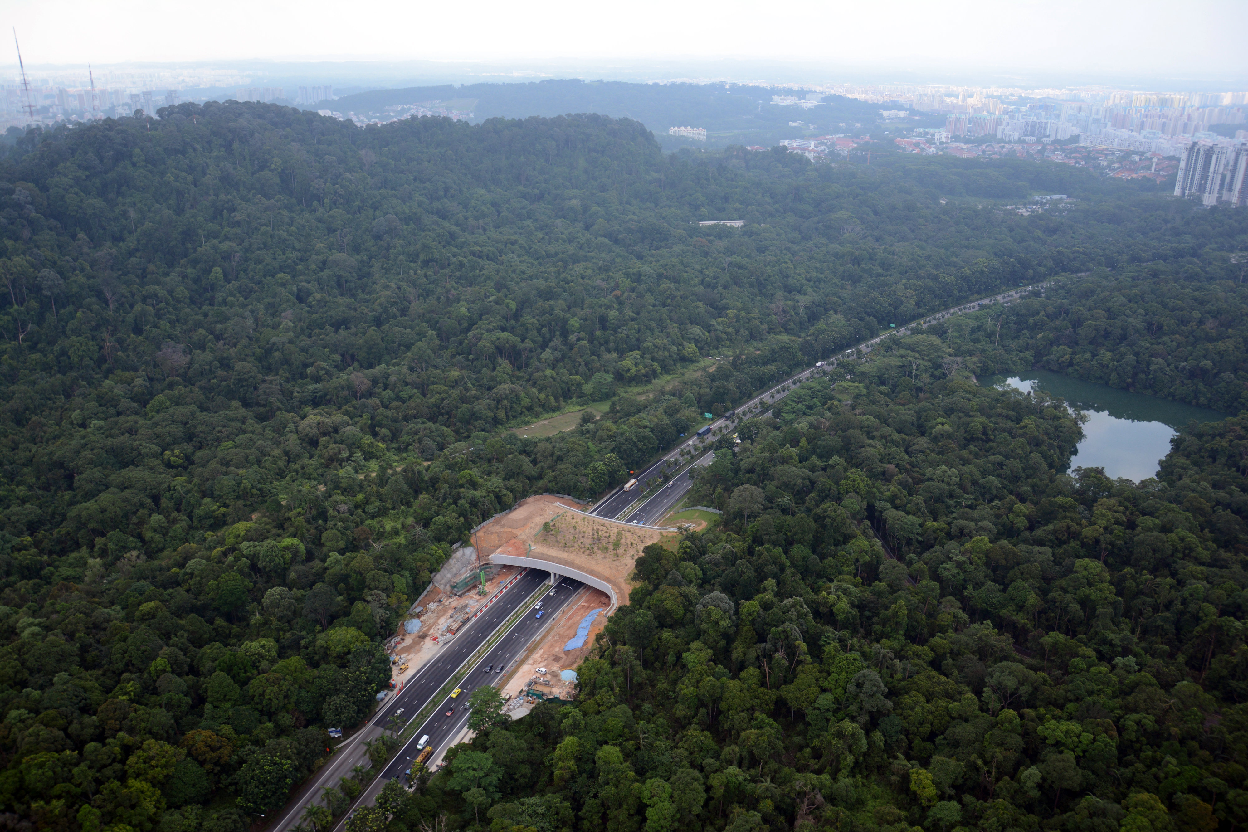
    Roadkill, we’ve all seen it on the roadside. It is just one very unfortunate outcomes of our extensive road networks. Roads, especially freeways and busy highways, also break apart habitats. When habitats are broken up into smaller pieces it weakens wildlife populations which need to move freely across landscapes for resources, refuge, and mates. Over long time scales, these fragmented habitats decrease species diversity, weaken species population gene pools, and can lead to extirpation (elimination of local population(s)) and extinction. As a result of numerous studies, ecologists have found one solution, wildlife crossings (aka green corridors or wildlife corridors). Wildlife crossings look like an underpass or overpass. However, they are filled with dirt and plants to look more natural. These crossings enable wildlife populations to move more freely, and safely, across landscapes all over the globe.

    Wildlife overpass over Singapore highway
    Figure \(\PageIndex{a}\): A newly constructed wildlife overpass over a Singapore highway. Image by Benjamin P. Y-H. Lee(opens in new window) (licensed under CC-BY-4.0(opens in new window))

    Populations are interacting and interbreeding groups of individuals from the same species in a common area. The study of population ecology focuses on population size and the factors that regulate population growth.


    • 3.1.1: Biological Organization
      This page is a summary of the hierarchy in nature.
    • 3.1.2: Population Distribution
      This page discusses the distribution patterns of populations, which include clumped, random, and uniform arrangements. Clumped distribution arises from uneven resource availability or social behaviors (e.g., elephants), random distribution lacks a specific pattern (e.g., dandelions), and uniform distribution occurs with even spacing due to resource scarcity or competition (e.g., saguaro cacti, penguins). These patterns enhance understanding of population interactions beyond just density.
    • 3.1.3: Population Size
      This page discusses the dynamics of populations influenced by factors such as environmental changes and resource competition. It highlights key characteristics like size and density, which affect genetic variation, adaptation, and interactions. The page also covers population size estimation methods, including quadrats for immobile organisms and mark-and-recapture for mobile species, noting that while these techniques yield estimates, actual numbers may be subject to errors and biases.
    • 3.1.4: Population Growth and Regulation
      This page covers population dynamics through models like exponential and logistic growth. Exponential growth is unrestricted (J-shaped curve), while logistic growth considers resource limits (S-shaped curve). It explains that population growth rates (r) hinge on birth and death rates. Additionally, the page discusses factors regulating growth, distinguishing between density-dependent (e.g., predation) and density-independent (e.g., natural disasters) influences.
    • 3.1.5: Life History
      This page explores life tables, which illustrate life expectancy and mortality rates by dividing populations into age groups. It highlights examples, like Dall mountain sheep, to show varying death rates at different ages and categorizes survivorship curves into Types I, II, and III. Furthermore, it contrasts r-selected species, which produce many offspring with minimal care, with K-selected species, which have fewer offspring but provide significant parental investment.
    • 3.1.6: Data Dive- Wildlife Corridors
      This page discusses the Sonoran Desert Conservation Plan, which started in 1999 to improve wildlife habitats and introduced wildlife corridors on SR 77. A monitoring plan was created to track species use of these corridors, supported by a graph showing an increase in wildlife crossings after two years.

    •  

    Attribution

    Modified by Erin Rempala. 

    Rachel Schleiger and Melissa Ha (CC-BY-NC(opens in new window))


    This page titled 3.1: Population Ecology is shared under a CC BY-NC-SA 4.0 license and was authored, remixed, and/or curated by Melissa Ha and Rachel Schleiger (ASCCC Open Educational Resources Initiative) .

    • Was this article helpful?