7.1.1: Geometric and Exponential Growth

INTRODUCTION

We will begin by developing a population model in discrete time. That is, we will treat time as if it moved in steps, rather than continuously. This allows us to use difference equations rather than differential equations, and thereby avoid the calculus. This assumption is realistic for many populations that have seasonal, synchronous reproduction. Strictly speaking, the discrete-time model represents geometric population growth. Later in the chapter, we will develop a continuous-time model, properly called an exponential model.

 

Model Development

To begin, we can write a very simple equation expressing the relationship between population size and the four demographic processes. Let:

• N_t represent the size or density of the population at some arbitrary time t (we will ignore the distinction between population size and population density)
• N_t+1 represent population size one arbitrary time-unit later
• B_t represent the total number of births in the interval from time t to time t + 1
• D_t represent the total number of deaths in the same time interval
• I_t represent the total number of immigrants in the same time interval
• E_t represent the total number of emigrants in the same time interval

 

Then we can write

 

For simplicity, this exercise ignores immigration and emigration. Our equation becomes

This equation is easy to understand but inconvenient for modeling. The problem lies in the use of “raw” birth and death rates (B_t and D_t). We have no obvious, biologically reasonable starting assumptions about these numbers. However, if we switch from raw birth and death rates to per capita birth and death rates, we can do some fruitful modeling.

 

Geometric (Discrete-Time) Model of Population Growth

A per capita rate is a rate per individual; that is, the per capita birth rate is the number of births per individual in the population per unit time, and the per capita death rate is the number of deaths per individual in the population per unit time. Per capita birth rate is easy to understand, and seems a reasonable thing to model because reproduction (giving birth) is something individuals rather than whole populations do. Per capita death rate may seem strange at first; after all, an individual can die only once. But remember, this rate is calculated per unit time. You can think of per capita birth and death rates as each individual’s probability of giving birth or dying in a given unit of time.

Keeping in mind that per capita rates are per individual rates, we can translate the raw rates B_t and D_t into per capita rates, which we will represent with lower-case letters (b_t and d_t) to distinguish them from the raw numbers. To calculate per capita rates, we divide the raw numbers by the population size. Thus,

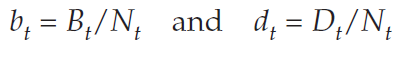
Conversely,

 

Now we can rewrite our model in terms of per capita rates:

Perhaps this seems to have gotten us nowhere, but it turns out to be a very informative model if we make one further assumption. Let us assume, just to see what happens, that per capita rates of birth and death remain constant over time. In other words, let us assume that average number of births per unit time per individual in the population and the average risk of dying per unit time remain unchanged over some period of time. What will happen to population size?

Because we assume constant per capita birth and death rates, we can make one further minor modification to our equation by leaving off the time subscripts on b and d:

At this point, you’re probably thinking that this assumption is unrealistic—that per capita rates of birth and death are likely to change over time for a variety of reasons. You are quite correct, but the model is still useful for three reasons:

• It provides a starting point for a more complex and realistic model in which per capita rates of birth and death do change over time.
• It is a good heuristic model—that is, it can lead to insights and learning despite its lack of realism.
• Many populations do in fact grow as predicted by this model, under certain conditions and for limited periods of time.

 

You may also wonder why we use this complex model (Equation 1) rather than the simpler forms of the geometric and exponential models presented in most textbooks (and developed here beginning with Equation 2). We prefer Equation 1 for three reasons:

• It emphasizes the roles of per capita birth and death rates rather than the more abstract quantities R or r (explained later).
• It allows you to manipulate per capita birth and death rates directly and separately, and discover that neither alone, but rather the difference between them, determines population growth rate.
• It allows you to discover that the per capita rate of population growth (DN_t/N_t) is a constant, which you can then relate to R (and r if desired).

 

Because per capita birth and death rates do not change in response to the size (or density) of the population, this model is said to be density-independent.

 

We can further simplify Equation 1 by factoring N_t out of the birth and death terms:

 

The term (b – d) is so important in population biology that it is given its own symbol, R. Thus R = b – d, and is called the geometric rate of increase. Substituting R for (b – d) gives us

To further define R, we can calculate the rate of change in population size, DNt, by subtracting

N_t from both sides of Equation 2:

Because DN_t = N_t+1 – N_t, we can simply write

In words, the rate of change in population size is proportional to the population size, and the constant of proportionality is R.

We can convert this to per capita rate of change in population size if we divide both sides by Nt:

In other words, the parameter R represents the (discrete-time) per capita rate of change in the size of the population.

Moving on, we can simplify Equation 2 (N_t+1 = N_t + RN_t) even further by factoring Nt out of the terms on the right-hand side, to get

The quantity (1 + R) is often given its own symbol, l (lambda), and its own name: the finite rate of increase. Substituting l, we can write

The quantity λ can be very useful in analyzing real population data. Some additional algebra will show us how.

 

If we divide both sides of Equation 5 by N_t, we get

In words, λ is the ratio of the population size at one time to its size one time-unit earlier. We can calculate λ from population counts at successive times, even if we do not know per capita rates of birth and death.

In Equations 2 and 5, we showed how to calculate the size of the population one time unit into the future. What if you wanted to know how big the population will be at some distant future time? You could carry out the one-time-step calculations many times, until you arrived at the desired answer. But there is also a shortcut. Population size at time 1 is λ¹N₀, at time 2 it is λ²N₀, and at time 3 it is λ³N₀. In general, we can write

This expression may strike you as rather abstract. One way to understand its impact is to use Equation 7 to calculate doubling time (t_double)—that is, the time required for the population to double in size. If we plug the doubling time into Equation 7, we get

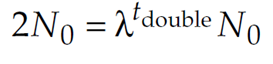
We can derive doubling time by exploiting the fact that the population at time t_double is, by definition, twice the population at time 0:

Substituting 2N₀ for N_t double gives us

If we divide both sides by N₀, we get

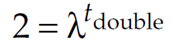
Taking the logarithm of both sides gives us

Dividing both sides by lnλ, we get

What does this mean? Suppose R = 0.1 individuals/individual/year. Therefore, λ = 1 + R = 1.1. This implies that the population increases by 10% per year, which doesn’t sound like much. But, if you plug this value of λ into Equation 8, you’ll find that the population doubles in about 7.27 years, which seems more impressive.

You may be wondering how a population that grows in discrete intervals of a year can double in a non-integer number of years. It can’t, of course. This calculation really means that the population will not quite double in 7 years, and will more than double in 8 years.

 

Exponential (Continuous-Time) Model of Population Growth

Population growth can also be modeled in continuous time, which is more realistic for populations that reproduce continuously, rather than seasonally. Continuous-time models also allow use of the calculus, which provides many powerful analytical tools. Here, we will eschew the calculus, and simply present some results.

Most textbooks begin with the continuous-time analog of Equation 3:

The left-hand side of Equation 9 represents the instantaneous rate of change in population size, which is different from the rate of change over some discrete time interval, DNt /Nt, that we looked at in Equation 7. Therefore, we use a lowercase r to distinguish the continuous-time exponential model from the discrete-time geometric model. The symbol r is called the instantaneous rate of increase or the intrinsic rate of increase. The parameters r and R are not equal, although they are related, as we will show below.

 

As we did with the discrete-time model, we can calculate the per capita rate of population growth by dividing both sides of Equation 9 by N:

You can use the calculus to operate on Equation 10 and calculate the size of the population at any time. We will spare you the derivation, but the resulting equation is

where e is the root of the natural logarithms (e ~ 2.71828).

You can derive the relationship between r and R as follows. Suppose we start two populations with the same initial number of individuals, N₀, and both grow at the same rate. However, one grows in continuous time and the other grows in discrete time. Because they grow at the same rate, at some later time, t, they will have reached the same size, N_t. If we write the discrete-time population on the left and the continuous-time population on the right we can derive as follows:

 

 

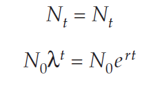
So, we can convert back and forth between continuous-and-discrete time models. Remember that λ = 1 + R.

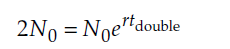
Suppose we have a population growing in continuous time with some value of r, and a population growing in discrete time with the same value of R, i.e., r = R. Which will grow faster? As we did with the geometric model, we can derive the doubling time for the exponential model (Gotelli 2001). We begin with Equation 11, and plug in tdouble:

Substituting 2N₀ for N_tdouble, we get

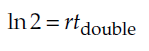
Dividing both sides by N₀ gives us

and taking the natural logarithm of both sides yields

Finally, we divide both sides by r, and rearrange, to get

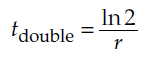
Parallel to our earlier example, let us suppose r = 0.1 individuals/individual/year. As before, this implies a 10% annual increase in the population, but now this increase occurs continuously rather than in discrete time intervals. How long does it take for this population to double? Plugging in the value 0.1 for r yields a doubling time of 6.93 years, somewhat faster than indicated by the geometric model.

 

EXPLORE THIS MODEL

Before moving on to the next section, explore this Exponential Growth Shiny App  developed by Dr. Aaron Howard to better understand how changes to the initial population size (N) and the population growth rate (r) impact population size over time.

 

SECTION SOURCE

Donovan, T. M. and C. Welden. 2002. Spreadsheet exercises in ecology and evolution. Sinauer Associates, Inc. Sunderland, MA, USA.

LITERATURE CITED

Gotelli, N. J. 2001. A Primer of Ecology, 3rd Edition. Sinauer Associates, Sunderland, MA.