
10.6: Projecting population growth
- Page ID
- 81284
Predicting changes in population size using lambda
Once we have a value for and the current size of the population from a complete census, we can estimate the future size of the population.
Recall that we arrived at lambda previously by setting up this equation
\[N_{t+1}/N_t=\lambda=\phi+b \nonumber\]
Where is \(\phi\) the survival rate of adults, and \(b\) is the number of offspring produced per adult that live to reproduce themselves.
We can rearrange this equation for making projections like this:
\[N_{t+1} =\lambda*N_t \nonumber\]
\(N_{t+1}/N_t= \lambda \) indicates that our concept of lambda is based on the ratio of two population sizes. Let’s start with this:
\[N_{t+1}/N_t=\lambda\nonumber\]
Now multiple both sizes by \(N_t\)
\[N_{t+1}/N_t*N_t=\lambda*N_t \nonumber\]
\(N_t\) cancels out from the left side and we get
\[N_{t+1}=\lambda*N_t \nonumber\]
This tells us that the population size next year \((N_{t+1})\) can be calculated as \(\lambda*(current.population.size)\).
Case Study: Projecting the number of Kirtland's Warblers
In 1990 it was estimated that there were 265 KIWA males with territories. If \[\lambda] = 1.3 as we calculated earlier, we’d predict that in 1991 the population size would be
\[N_{1991}=\lambda*N_{1990} \nonumber\]
\[N_{1991}=1.3*265=344.5 \nonumber\]
So we’d predict there to be 344 or 345 birds in 1991 (you can’t have 0.5 of an organism. Indeed, researchers observed 347 birds.
We can repeat this using our estimate for 1991 to estimate 1992 and so on. When you plug the output of an equation (eg N1991=344) back into itself repeatedly this is called recursion.
The equation
\[N_{t+1}=\lambda*N_t \nonumber\]
is therefore sometimes referred to as a recursion equation. (Similar terms are iterate and iteratively.)
Exponential population growth
If you take the population size of 344 KIWA from our last calculation and plug it back into the population growth equation like this to estimate the number of warblers in the next year, 1992:
\[N_{1992}=1.3*344=447.2 \nonumber\]
The estimated population the following year will be about 447 KIWA males. In reality, there were 497 males counted, so our projection is a bit low
If you repeat this process of plugging the results of one calculation into the next calculation 8 more times (for 10 total years of population change) we can project the population size for a decade. Note the convex, upward curvature of the line. This upward, accelerating curve is an exponential growth curve. Exponential growth occurs when something increases by multiplication. This is in contrast to arithmetic growth, which occurs when something increases by addition.
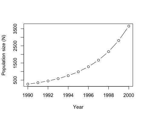
Figure \(\PageIndex{1}\): Exponential growth increases by multiplication and accelerates the population size over time without limit.
Many things in the world change arithmetically. For example, if you are being paid by the hour to do a job and don't have to work an entire day, the amount you earn increases arithmetically. Some populations can grow arithmetically if individuals from other populations are being introduced intentionally to the population. For example, the Peregrine falcon (Falco peregrinus) has a geographic range that encompases the entire world. However, due to the impacts of pesticides such as DDT the falcon was almost extirpated from many places in the United States. In addition to banning DDT, falcon populations were restored by taking young falcons from large populations and introducing them to smaller populations. If 10 falcons were introduced each year to a population, the fixed number of new individuals results in arithmetic contribution to growth.
In contrast to the fixed increases of arithmetic growth, exponential growth occurs multiplicatively - that is, by multiplying the current population size by a growth rate. If a population of falcons has 100 birds and a growth rate of 1.10, then it's population size the next year is 100*1.10 = 110. The next year if the growth rate is still 1.10 the population would be 110*1.10 = 121. Therefore the first time step the change in population size (delta N) was 10 individuals (110-100 = 10), while over the second time step delta N was 11 individuals (121-110 = 11). If we projected a third year the population would be 121*1.10 = 133.1. Delta N is therefore increasing each year from 10, to 11, to about 12. This is why we use the term "accelerating" to describe this type of growth: each year the amount of change increases.

Figure \(\PageIndex{2}\): Male peregrine falcon (Falco peregrinus) in Humber Bay Park West in Toronto. "Falco peregrinus" by Сапсан is licensed under CC BY-SA 3.0.
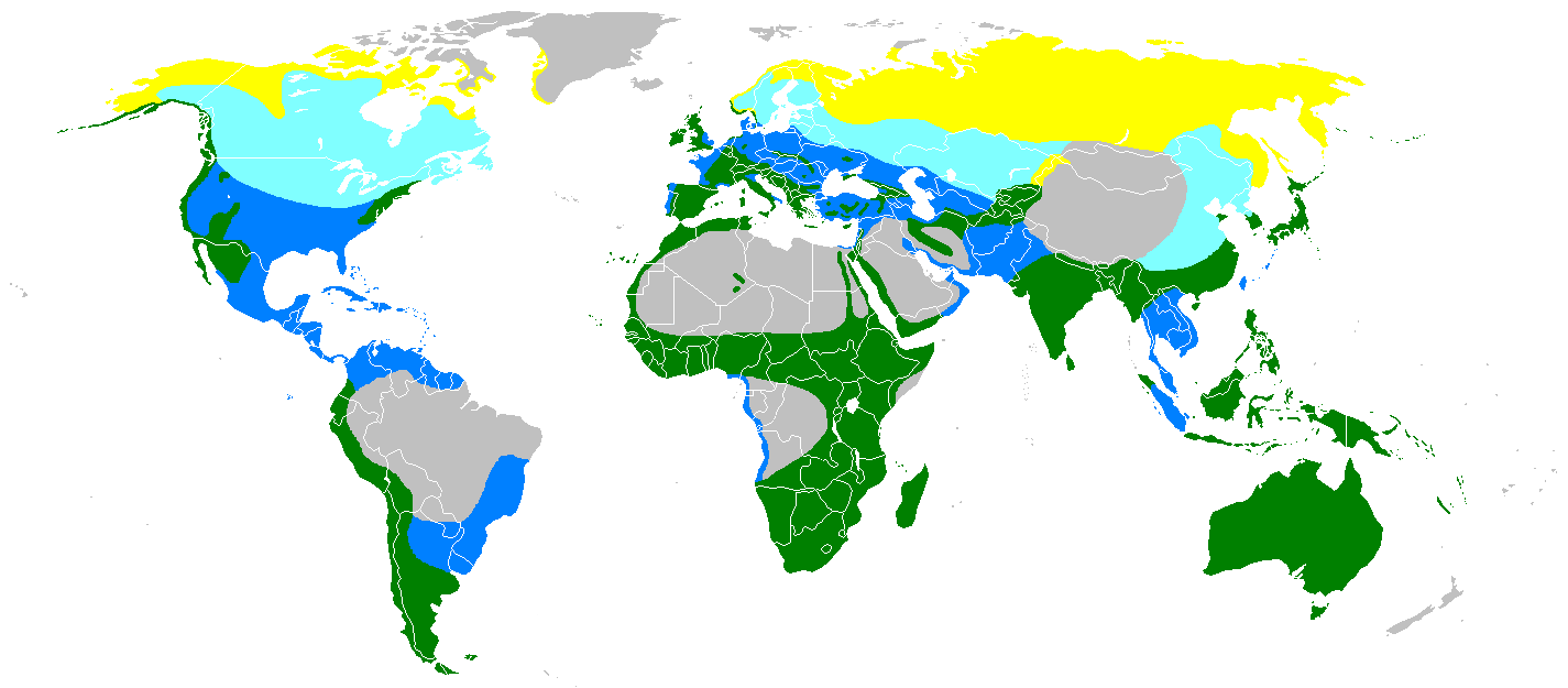
Figure \(\PageIndex{3}\): The peregrine falcon's range covers most of the world, besides some areas of Africa, the Arabian Peninsula, South America, Greenland, and Asia. The birds' large home range allows for alternative options from limiting factors. "Range map for Falco peregrinus (including F. (p.) pelegrinoides, the Barbary falcon)" by MPF is licensed under CC BY-SA 3.0.
Case study: The Montserrat Oriole
The Montserrat Oriole (Icterus oberi) is a relative of the Baltimore Oriole (Icterus galbula). While the Baltimore Oriole occurs throughout eastern and central North America, the Montserrat Oriole lives only on the Caribbean island of Montserrat. Montserrat is a small volcanic island that is only about 10 miles long and 7 miles wide and lies east of Puerto Rico and north of Barbados. Since the Montserrat Oriole only occurs on the island of Montserrat. It therefore is an entirely closed population. The Montserrat Oriole is therefore called a single-island endemic species, like the Cozumel Thrasher.
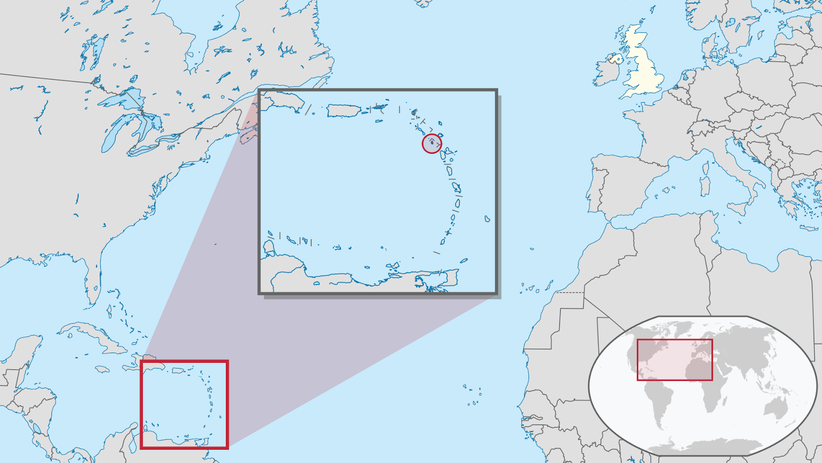
Figure \(\PageIndex{4}\): The red box identifies Montserrat. "Location of Montserrat" by TUBS is licensed under CC BY-SA 3.0 / adapted from original.
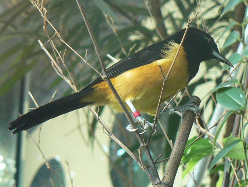
Figure \(\PageIndex{5}\): The Montserrat Oriole is only present on the island of Montserrat in a closed population. "Male Montserrat Oriole (Icterus oberi), London Zoo" by Neil Phillips is licensed under CC BY 2.0.
Volcanic activity in the 1990s on Montserrat has destroyed its forest habitat and rained ash down across the island, destroying nests and killing the birds’ insect prey. N was therefore negative due to a low number of births of new birds and a high death rate of members of the existing population due to starvation. The species is therefore threatened with extinction - death of all members of the population. Biologists have become very interested in determining how many orioles are left on the island and what is happening with the population.
The Montserrat Oriole population size is small, but researchers have never been able to determine how many there are. What they have done, however, is marked a subset of adult orioles with bird bands and re-captured them each year to estimate survival rates. They have also found some nests and determined how many baby orioles are born per nest, and what the survival rate is for those birds until they are one year old and can breed. This gives an estimate of b.
Survival for the Montserrat Oriole is currently around 70%, or 0.70. This means that if there were 100 birds banded, 70 of them survived to the following year. Alternatively, we can think of this in terms of probability: a single bird banded this year has a 70% chance of surviving to the next year to be re-captured.
The birth rate is tricky to estimate for a number of reasons; incorporating both the number of Orioles that hatch from eggs and their probability of surviving for one year until they can reproduce, the birth rate (b) is about 0.42. The population growth rate is therefore
\[\lambda=0.70+0.42 \nonumber\]
\[\lambda=1.12 \nonumber\]
Since \(\lambda \) >1 we’d predict that the population of Orioles will be growing. As before, we aren’t actually counting all the birds, but instead using demographic rates to estimate lambda.
In 2012 it was estimated that there might be as few as 300 Orioles on the island. If \(\lambda = 1.12 \) as we calculated above, we’d predict that in 2013 the population size would be
\[N_{2013}=\lambda*N_{2012} \nonumber\]
\[N_{2013}=1.12*300=336 \nonumber\]
In 2001 a second, very small population of Montserrat Orioles was found very near to the crater of the volcano on the island. Researchers haven’t studied this population much, but they estimate that there were about 100 birds in 2020.
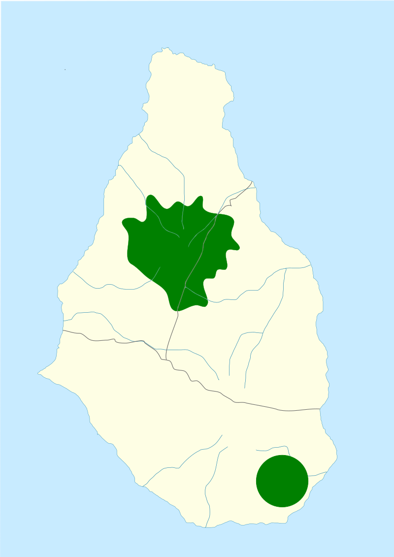
Figure \(\PageIndex{6}\): Green spots on the island of Montserrat identify habitats. "Range map of Montserrat Oriole (Icterus oberi)" by Cephas is licensed under CC BY-SA 4.0.
If you start with 100 Orioles and you estimate that for this population is 1.10 you can start with this equation
\[N_{t+1}=\lambda*Nt \nonumber\]
We can make this more specific with subscripts:
\[N_{2021}=\lambda*N_{2020} \nonumber\]
then plug in the values \(lambda= 1.10\) and N = 100
\[N_{2021}=1.1*100 \nonumber\]
and get the project population the following year
\[N_{2021}=110 \nonumber\]
So, if you have 100 orioles in 2020 you’d expect to have 2021 next year.
Exponential population growth of Orioles
If you take the population size of 110 orioles from our last calculation and plug it back into the population growth equation you can estimate the number of orioles in next year, 2022:
\[N_{2022}=1.1*110 \nonumber\]
the estimated population the following year will be 121 orioles.
\[N_{2022}=121 \nonumber\]
If you repeat this 8 more times (for 10 total years of population change since 2020) you will see a graph like the one below. Note the slight, convex, upward curvature of the line.
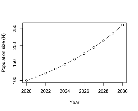
Figure \(\PageIndex{7}\): Exponential growth models can be used to graph the predicted population sizes of species.
Contributors and Attributions
This chapter was written by NL Brouwer (University of Pittsburgh)