12.7: Predator satiation and starvation

Figure \(\PageIndex{1}\). Predators satiated versus sick and starving.

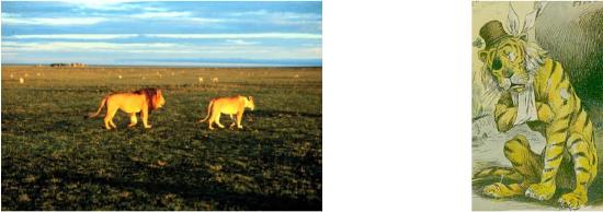
In the original Lotka–Volterra formulation, doubling the number of prey in the environment doubles the number of prey taken. The same is true in the equivalent \(r\,+\,sN\) formulation explored above. While this may be reasonable at low prey densities, eventually the predators become satiated and stop hunting, as in the image at left in Figure \(\PageIndex{1}\). Satiation will therefor truncate the predator growth curve at some maximum rate, as at right in Figure \(\PageIndex{2}\).

Figure \(\PageIndex{2}\). Predator growth truncated at a maximum number of prey taken per predator per unit of time.

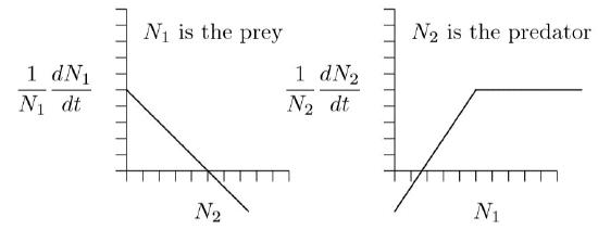
In the opposite direction, if prey are not available, the predator population starves, as in the sad image at right in Figure \(\PageIndex{1}\). As indicated by a negative vertical intercept in Figures \(\PageIndex{2}\) and elsewhere, the population does not reach a maximum rate of decline. In the complete absence of prey, vertebrate predators decline more and more rapidly, reaching extinction at a definite time in the future, as induced by the increasingly large rates of decline shown in the right part of Figure \(\PageIndex{3}\). This is a different kind of singularity that can actually occur in a finite time.

Figure \(\PageIndex{3}\). Vertebrate predators with asymptotic rates of consumption.

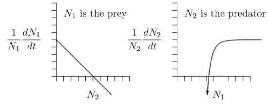
As an exercise and illustration, let us create a predator– prey system in which the predators become satiated and reach a maximum growth rate, but for which there is no maximum death rate in the absence of prey, and see where it leads.

For predators, we want to mimic the shape at right in Figure \(\PageIndex{3}\). This has the shape of a hyperbola, \(y\,=\,1/x\), but reflected about the horizontal axis and shifted upwards. The equation would be \(y\,=\,a\,-\,b/x\), where \(a\) and \(b\) are positive constants. When \(x\) approaches infinity, the term \(b/x\) goes to zero and \(y\) therefore approaches \(a\). It crosses the horizontal axis where \(x\,=\,b/a\), then heads downward toward minus infinity as \(x\) declines to zero. Such a curve has the right general properties.

The predator equation can therefore be the following, with \(r_1\) for \(a\), \(s_{1,2}\) for \(−b\), and \(N_1\) for \(x\).

\(\frac{1}{N_2}\frac{dN_2}{dt}\,=\,r_2\,+\,s_{2,1}\frac{1}{N_1}\)

When there are ample prey \(N_1\) will be large, so the term \(s_{2,1}/N_1\) will be small and the predator growth rate will be near \(r_2\). As prey decline, the term \(s_{2,1}/N_1\) will grow larger and larger without limit and, since \(s_{2,1}\) is less than zero, the predator growth rate will get more and more negative, also without limit.

What about the prey equation? The important point here is that predators become satiated, so the chance of an individual prey being caught goes down as the number of prey in the environment goes up. So instead of a term like \(s_{1,2}N_2\) for the chance that an individual prey will be taken, it would be more like \(s_{1,2}\,N_2/N_1\).

\(\frac{1}{N_1}\frac{dN_1}{dt}\,=\,r_1\,+\,s_{1,2}\frac{N_2}{N_1}\,+\,s_{1,1}N_1\)

In other words, the rate of prey being taken increases with the number of predators in the environment, but is diluted as there are more and more prey and predators become satiated. Eventually, with an extremely large number of prey in the area relative to the number of predators, the effect of predators on each individual prey becomes negligible. This creates the following predator–prey system, which takes satiation and starvation into account:

\(\frac{1}{N_1}\frac{dN_1}{dt}\,=\,r_1\,+\,s_{1,2}\frac{N_2}{N_1}\,+\,s_{1,1}N_1\)

\(\frac{1}{N_2}\frac{dN_2}{dt}\,=\,r_2\,+\,s_{2,1}\frac{1}{N_1}\)

This system could be criticized because it is not “mass balanced.” In other words, one unit of mass of prey does not turn directly into a specific amount of mass of predators. But this is not a simple molecular system, and it at least fits more closely the realities of predator and prey behavior.

In any case, keep in mind that \(s_{1,1}\) is less than 0, to reflect limitation of prey due to crowding and other effects; \(s_{2,2}\) is equal to 0, assuming the predator is limited only by the abundance of prey; \(s_{1,2}\) is less than 0 because the abundance of predators decreases the growth of prey; and \(s_{2,1}\) is also less than 0 because as the number of prey decreases there is an increasingly negative effect on the growth of the predator.

The next step is to examine the isoclines for this new set of equations, making a phase-space graph with \(N_1\) on the horizontal axis versus \(N_2\) on the vertical. Where does the prey growth, \(\frac{1}{N_1}\frac{dN_1}{dt}\), cease? Working through some algebra, it is as follows:

\(\frac{1}{N_1}\frac{dN_1}{dt}\,=\,0\,=\,r_1\,-\,s_{1,2}\frac{N_2}{N_1}\,-\,s_{1,1}N_1\)

\(\Rightarrow\,\,s_{1,2}\frac{N_2}{N_1}\,=\,r_1\,-\,s_{1,1}N_1\)

\(\Rightarrow\,\,N_2\,=\frac{r_1}{s_{1,2}}\,N_1\,-\frac{s_{1,1}}{s_{1,2}}\,N_1^2\)

Similarly, where does the predator growth, \(\frac{1}{N_2}\frac{dN_2}{dt}\), cease for the same phase-plane? Let's follow similar algebra:

\(\frac{1}{N_2}\frac{dN_2}{dt}\,=\,0\,r_2\,+\,s_{2,1}\frac{1}{N_1}\)

\(\Rightarrow\,\,-r_2\,=\,s_{2,1}\frac{1}{N_1}\)\

\(\Rightarrow\,\,N_1\,=\,-\frac{s_{2,1}}{r_2}\)

This predator isocline is simply a vertical line, as before in Figures 12.4.2 and following figures. But note that the prey curve has the form of an inverted parabola—a hump, as graphed for two cases in Figure \(\PageIndex{4}\).

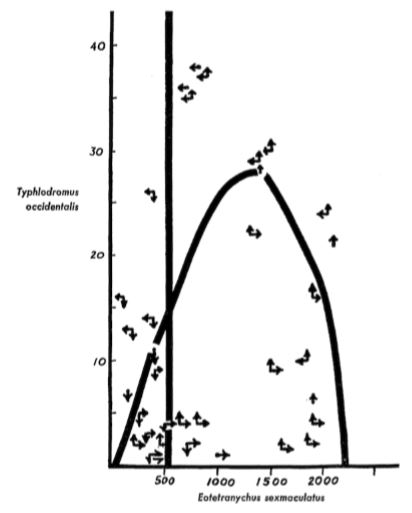
Remarkably, this formulation of predator–prey equations closely matches what earlier researchers deduced logically and graphically, when computers were slow or not yet available. If you want to better understand the shape of the prey curve, read Rosenzweig’s 1969 paper entitled “Why the prey curve has a hump.” For interest, his hand-drawn published figure with experimental data points is reproduced in Figure \(\PageIndex{5}\).

Rosenzweig pointed out a paradoxical effect, which he called “the paradox of enrichment.” At left in Figure \(\PageIndex{5}\), the prey have a relatively low carrying capacity, with \(K\,=\,−r_1\,/\,s_{1,1}\) about halfway along the horizontal axis. If you analyze the flow around the red dot that marks the equilibrium point to the right of the hump, or run a program to simulate the equations we just derived, you will find that the populations spiral inward. The equilibrium is stable.

Figure \(\PageIndex{4}\). The paradox of enrichment, Rosenzweig, AmNat 1969.

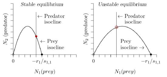
The paradox is this: if you try to improve conditions for the prey by increasing their carrying capacity—by artificially providing additional food, for example— you can drive the equilibrium to the left of the hump, as in the right part of Figure \(\PageIndex{4}\). Around the equilibrium marked by the red circle, the populations spiral outward. The system has become unstable.

This is a warning from ecological theory. In conservation efforts where predators are present, trying to enhance a prey population by increasing its carrying capacity could have the opposite effect. This is not to say that efforts to enhance prey populations should not be undertaken, only that they should proceed with appropriate caution and study.

Figure \(\PageIndex{5}\). Rosenzweig’s original 1969 graph with phase-space arrows, interpreting Huffaker’s 1958 experiments with mites.