8.1: Dynamics of two Interacting Species

In the first part of this book you’ve seen the two main categories of single-species dynamics—logistic and orthologistic, with exponential growth being an infinitely fine dividing line between the two. And you’ve seen how population dynamics can be simple or chaotically complex.

Moving forward you will see three kinds of two-species dynamics—mutualism, competition, and predation—and exactly forty kinds of three-species dynamics, deriving from the parameters of the population equations and their various combinations.

To review, the population dynamics of a single species are summarized in the following equation.

\[\frac{1}{N}\frac{dN}{dt}\,=\,r\,+\,sN\]

Here parameter r is the “intrinsic growth rate” of the species— the net rate at which new individuals are introduced to the population when the population is vanishingly sparse, and s is a “density dependence” parameter that reflects how the size of the population affects the overall rate. Parameter s is key. If s is negative, the population grows “logistically,” increasing to a “carrying capacity” of −r /s, or decreasing to that carrying capacity if the population starts above it. If s is positive, then the population grows “orthologistically,” increasing ever faster until it encounters some unspecified limit not addressed in the equation. Exponential growth is the dividing line between these two outcomes, but this would only occur if s remained precisely equal to zero.

How should this single-species equation be extended to two species? First, instead of a number N for the population size of one species, we need an N for each species. Call these N₁ for species 1 and N₂ for species 2. Then, if the two species do not interact at all, the equations could be

\[\frac{1}{N_1}\frac{dN_1}{dt}\,=\,r_1\,+\,s_{1,1}\,N_1\]

\[\frac{1}{N_2}\frac{dN_2}{dt}\,=\,r_2\,+\,s_{2,2}\,N_2\]

Here r₁ and r₂ are the intrinsic growth rates for N₁ and N₂, respectively, and s_1,1 and s_2,2 are the density dependence parameters for the two species. (The paired subscripts in the two-species equations help us address all interactions.)

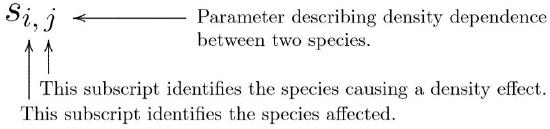
There are thus four possible s_i,j parameters here:

• s_1,1 : How density of species 1 affects its own growth.
• s_1,2 : How density of species 2 affects the growth of species 1.
• s_2,1 : How density of species 1 affects the growth of species 2.
• s_2,2 : How density of species 2 affects its own growth.

With these parameters in mind, here are the two-species equations. The new interaction terms are in blue on the right.

\[\frac{1}{N_1}\,\frac{dN_1}{dt}\,=\,r_1\,+\,s_{1,1}N_1\,+\,\color{blue}{s_{1,2}N_2}\]

\[\frac{1}{N_2}\,\frac{dN_2}{dt}\,=\,r_2\,+\,s_{2,2}N_2\,+\,\color{blue}{s_{2,1}N_1}\]

In the single-species equations, the sign of the s term separates the two main kinds of population dynamics—positive for orthologistic, negative for logistic. Similarly, in the two-species equations, the signs of the interaction parameters s_1,2 and s_2,1 determine the population dynamics.

Two parameters allow three main possibilities—(1) both parameters can be negative, (2) both can be positive, or (3) one can be positive and the other negative. These are the main possibilities that natural selection has to work with.

Figure \(\PageIndex{1}\). Both interaction parameters negative, competition.

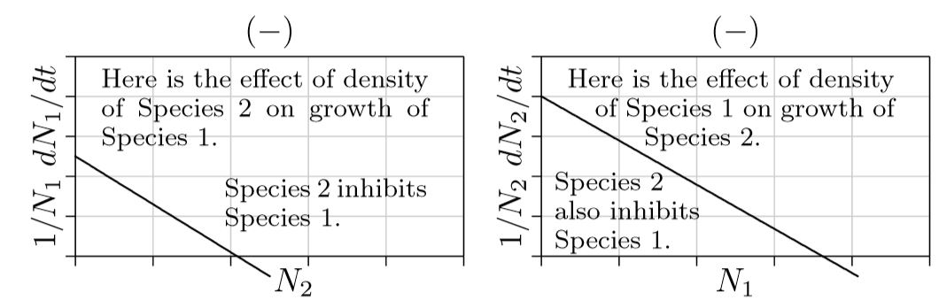
Competition. First consider the case where s_1,2 and s_2,1 are both negative, as in Figure \(\PageIndex{1}\).

Figure \(\PageIndex{2}\). Time course of competition, one example.

For a single species, parameter s being negative causes the population to approach a carrying capacity. The same could be expected when parameters s_1,2 and s_2,1 are both negative—one or both species approach a carrying capacity at which the population remains constant, or as constant as external environmental conditions allow.

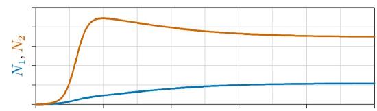
One example is shown in Figure \(\PageIndex{2}\), where the population of each species is plotted on the vertical axis and time on the horizontal axis. Here Species 2, in red, grows faster, gains the advantage early, and rises to a high level. Species 1, in blue, grows more slowly but eventually rises and, because of the mutual inhibition between species in competition, drives back the population of Species 2. The two species eventually approach a joint carrying capacity.

In other cases of competition, a “superior competitor” can drive the other competitor to extinction—an outcome called “competitive exclusion.” Or, either species can drive the other to extinction, depending on which gains the advantage first. These and other cases are covered in later chapters.

In any case, when both interaction terms s_1,2 and s_2,1 are negative, in minus–minus interaction, each species inhibits the other’s growth, which ecologists call the “interaction competition”.

Mutualism. The opposite of competition is mutualism, where each species enhances rather than inhibits the growth of the other. Both s_1,2 and s_2,1 are positive.

Figure \(\PageIndex{3}\): Both interaction parameters positive, mutualism.

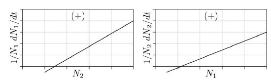
Depicted in Figure \(\PageIndex{3}\) is a form of “obligate mutualism,” where both species decline to extinction if either is not present. This is analogous to a joint Allee point, where the growth curves cross the horizontal axis and become negative below certain critical population levels. If this is not the case and the growth curves cross the vertical axis, each species can survive alone; this is called “facultative mutualism,” and we’ll learn more about it in later chapters.

For now, the important point is how mutualistic populations grow or decline over time. A single species whose density somehow enhances its own rate of growth becomes orthologistic, increasing ever more rapidly toward a singularity, before which it will grow so numerous that it will be checked by some other inevitable limit, such as space, predation, or disease.

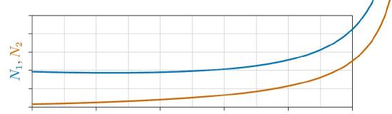
It turns out that the dynamics of two species enhancing each other’s growth are similar to those of a single species enhancing its own growth. Both move to a singularity at ever increasing rates, as illustrated earlier in Figure 4.2.1 and below in Figure \(\PageIndex{4}\). Of course, such growth cannot continue forever. It will eventually be checked by some force beyond the scope of the equations, just as human population growth was abruptly checked in the mid-twentieth century— so clearly visible earlier in Figure 6.3.1.

Figure \(\PageIndex{4}\): Time course of unchecked mutualism

Predation. The remaining possibility for these two-species equations is when one interaction parameter si,j is positive and the other is negative. In other words, when the first species enhances the growth of the second while the second species inhibits the growth of the first. Or vice versa. This is “predation,” also manifested as parasitism, disease, and other forms.

Think about a predator and its prey. The more prey, the easier it is for predators to catch them, hence the easier it is for predators to feed their young and the greater the predator’s population growth. This is the right part of Figure \(\PageIndex{5}\). The more predators there are, however, the more prey are captured; hence the lower the growth rate of the prey, as shown on the left of the figure. N₁ here, then, represents the prey, and N₂ represents the predator.

Figure \(\PageIndex{5}\). Interaction terms of opposite signs, predation.

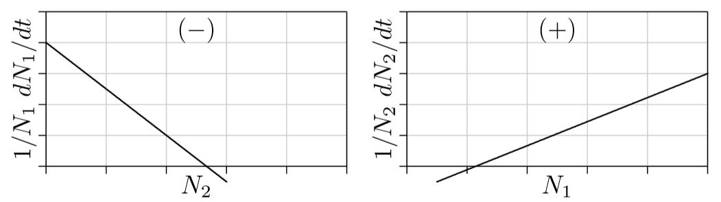
Prey can survive on their own, without predators, as reflected on the left in positive growth for N₁ when N₂ is 0. Predators, however, cannot survive without prey, as reflected on the right in the negative growth for N₂ when N₁ is 0. This is like an Allee point for predators, which will start to die out if the prey population falls below this point.

The question here is this: what will be the population dynamics of predator and prey through time? Will the populations grow logistically and level off at a steady state, as suggested by the negative parameter s_1,2, or increase orthologistically, as suggested by the positive parameter s_2,1?

Actually, they do both. Sometimes they increase faster than exponentially, when predator populations are low and growing prey populations provide ever increasing per capita growth rates for the predator, according to the right part of Figure \(\PageIndex{5}\). In due time, however, predators become abundant and depress prey populations, in turn reducing growth of the predator populations. As shown in Figure \(\PageIndex{6}\), the populations oscillate in ongoing tensions between predator (red line) and prey (blue line).

Figure \(\PageIndex{6}\). Time course of predation.

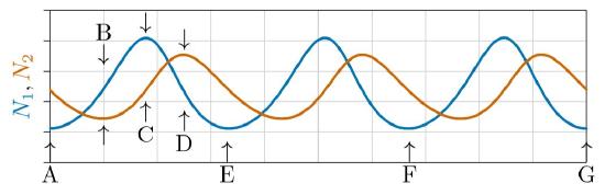
Examine this figure in detail. At the start, labeled A, the prey population is low and predators are declining for lack of food. A steady decline in the number of predators creates better and better conditions for prey, whose populations then increase orthologistically at ever accelerating per capita rates as predators die out and conditions for prey improve accordingly.

But then the situation turns. Prey grow abundant, with the population rising above the Allee point of the predator, at B. The number of predators thus start to increase. While predator populations are low and the number of prey is increasing, conditions continually improve for predators, and their populations grows approximately orthologistically for a time.

Then predators become abundant and drive the growth rate of the prey negative. The situation turns again, at C. Prey start to decline and predator growth becomes approximately logistic, leveling off and starting to decline at D. By E it has come full circle and the process repeats, ad infinitum.

While Figure \(\PageIndex{6}\) illustrates the classical form for predator-prey interactions, other forms are possible. When conditions are right, the oscillations can dampen out and both predator and prey populations can reach steady states. Or the oscillations can become so wild that predators kill all the prey and then vanish themselves. This assumes some effectively-zero value for N₁ and N₂, below which they “snap” to zero. Or prey populations can become so low that predators all die out, leaving the prey in peace. Or both can go extinct. Or, in the case of human predators, the prey can be domesticated and transformed into mutualists. More on all such dynamics in later chapters.