30.4: Mendelian Traits

Last updated
Save as PDF

Page ID: 41190

\( \newcommand{\vecs}[1]{\overset { \scriptstyle \rightharpoonup} {\mathbf{#1}} } \) \( \newcommand{\vecd}[1]{\overset{-\!-\!\rightharpoonup}{\vphantom{a}\smash {#1}}} \)\(\newcommand{\id}{\mathrm{id}}\) \( \newcommand{\Span}{\mathrm{span}}\) \( \newcommand{\kernel}{\mathrm{null}\,}\) \( \newcommand{\range}{\mathrm{range}\,}\) \( \newcommand{\RealPart}{\mathrm{Re}}\) \( \newcommand{\ImaginaryPart}{\mathrm{Im}}\) \( \newcommand{\Argument}{\mathrm{Arg}}\) \( \newcommand{\norm}[1]{\| #1 \|}\) \( \newcommand{\inner}[2]{\langle #1, #2 \rangle}\) \( \newcommand{\Span}{\mathrm{span}}\) \(\newcommand{\id}{\mathrm{id}}\) \( \newcommand{\Span}{\mathrm{span}}\) \( \newcommand{\kernel}{\mathrm{null}\,}\) \( \newcommand{\range}{\mathrm{range}\,}\) \( \newcommand{\RealPart}{\mathrm{Re}}\) \( \newcommand{\ImaginaryPart}{\mathrm{Im}}\) \( \newcommand{\Argument}{\mathrm{Arg}}\) \( \newcommand{\norm}[1]{\| #1 \|}\) \( \newcommand{\inner}[2]{\langle #1, #2 \rangle}\) \( \newcommand{\Span}{\mathrm{span}}\)\(\newcommand{\AA}{\unicode[.8,0]{x212B}}\)

Mendel

Gregor Mendel identified the first evidence of inheritance in 1865 using plant hybridization. He recognized discrete units of inheritance related to phenotypic traits, and noted that variation in these units, and therefore variations in phenotypes, was transmissible through generations. However, Mendel ignored a discrepancy in his data: some pairs of phenotypes were not passed on independently. This was not understood until 1913, when linkage mapping showed that genes on the same chromosome are passed along in tandem unless a meiotic cross-over event occurs. Furthermore, the distance between genes of interest describes the probability of a recombination event occuring between the two loci, and therefore the probability of the two genes being inherited together (linkage).

Figure 30.3: A pedigree which shows the inheritance of some trait

Linkage Analysis

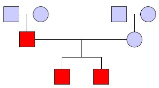
Historically, researchers have used the idea of linkage through linkage analysis to determine genetic variants which explain phenotypic variation. The goal is to determine which variants contribute to the observed pattern of phenotypic variation in a pedigree. Figure 30.3 shows an example pedigree in which squares are male individuals, circles are female individuals, couples and offspring are connected, and individuals in red have the trait of interest.

Linkage analysis relies on the biological insight that genetic variants are not independently inherited (as proposed by Mendel). Instead, meiotic recombination happens a limited number of times (roughly once per chromosome), so many variants cosegregate (are inherited together). This phenomenon is known as linkage disequilibrium (LD).

As the distance between two variants increases, the probability a recombination occurs between them increases. Thomas Hunt Morgan and Alfred Sturtevant developed this idea to produce linkage maps which could not only determine the order of genes on a chromosome, but also their relative distances to each other. The Morgan is the unit of genetic distance they proposed; loci separated by 1 centimorgan (cM) have 1 in 100 chance of being separated by a recombination. Unlinked loci have 50% chance of being separated by a recombination (they are separated if an odd number of recombinations happens between them). Since we usually do not know a priori which variants are causal, we instead use genetic markers which capture other variants due to LD. In 1980, David Botstein proposed using single nucleotide polymorphisms (SNPs), or mutations of a single base, as genetic markers in humans [4]. If a particular marker is in LD with the actual causal variant, then we will observe its pattern of inheritance contributing to the phenotypic variation in the pedigree and can narrow down our search.

The statistical foundations of linkage analysis were developed in the first part of the 20th century. Ronald Fisher proposed a genetic model which could reconcile Mendelian inheritance with continuous phenotypes such as height [10]. Newton Morton developed a statistical test called the LOD score (logarithm of odds) to test the hypothesis that the observed data results from linkage [26]. The null hypothesis of the test is that the recombination fraction (the probability a recombination occurs between two adjacent markers) \(\theta\) = 1/2 (no linkage) while the alternative hypothesis is that it is some smaller quantity. The LOD score is essentially a log-likelihood ratio which captures this statistical test:

\[\mathrm{LOD}=\frac{\log (\text { likelihood of disease given linkage })}{\log (\text { likelihood of disease given no linkage })}\nonumber\]

The algorithms for linkage analysis were developed in the latter part of the 20th century. There are two main classes of linkage analysis: parametric and nonparametric [34]. Parametric linkage analysis relies on a model (parameters) of the inheritance, frequencies, and penetrance of a particular variant. Let F be the set of founders (original ancestors) in the pedigree, let gi be the genotype of individual i, let \(\Phi_{i}\) be

Figure 30.4: Representing a particular pattern of inheritance as an inheritance vector

the phenotype of individual i, and let f(i) and m(i) be the father and mother of individual i. Then, the likelihood of observing the genotypes and phenotypes in the pedigree is:

\[L=\sum_{g_{1}} \ldots \sum_{g_{n}} \prod_{i} \operatorname{Pr}\left(\Phi_{i} \mid g_{i}\right) \prod_{f \in F} \operatorname{Pr}\left(g_{f}\right) \prod_{i \notin F} \operatorname{Pr}\left(g_{i} \mid g_{f(i)}, g_{m(i)}\right)\nonumber\]

The time required to compute this likelihood is exponential in both the number of markers being considered and the number of individuals in the pedigree. However, Elston and Stewart gave an algorithm for more efficiently computing it assuming no inbreeding in the pedigree [8]. Their insight was that conditioned on parental genotypes, offspring are conditionally independent. In other words, we can treat the pedigree as a Bayesian network to more efficiently compute the joint probability distribution. Their algorithm scales linearly in the size of the pedigree, but exponentially in the number of markers.

There are several issues with parametric linkage analysis. First, individual markers may not be informative (give unambiguous information about inheritance). For example, homozygous parents or genotyping error could lead to uninformative markers. To get around this, we could type more markers, but the algorithm does not scale well with the number of markers. Second, coming up with model parameters for a Mendelian disorder is straightforward. However, doing the same for non-Mendelian disorders is non-trivial. Finally, estimates of LD between markers are not inherently supported.

Nonparametric linkage analysis does not require a genetic model. Instead, we first infer the inheritance pattern given the genotypes and the pedigree. We then determine whether the inheritance pattern can explain the phenotypic variation in the pedigree.

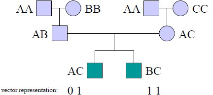
Lander and Green formulated an HMM to perform the first part of this analysis [20]. The states of this HMM are inheritance vectors which specify the result every meiosis in the pedigree. Each individual is represented by 2 bits (one for each parent). The value of each bit is 0 or 1 depending on which of the grand-parental alleles is inherited. Figure 30.4 shows an example of the representation of two individuals in an inheritance vector.

Each step of the HMM corresponds to a marker; a transition in the HMM corresponds to some bits of the inheritance vector changing. This means the allele inherited from some meiosis changed, i.e. that a recombination occurred. The transition probabilities in the HMM are then a function of the recombination fraction between adjacent markers and the Hamming distance (the number of bits which differ, or the number of recombinations) between the two states. We can use the forward-backward algorithm to compute posterior probabilities on this HMM and infer the probability of every inheritance pattern for every marker.

This algorithm scales linearly in the number of markers, but exponentially in the size of the pedigree. The number of states in the HMM is exponential in the length of the inheritance vector, which is linear in the size of the pedigree. In general, the problem is known to be NP-hard (to the best of our knowledge, we cannot do better than an algorithm which scales exponentially in the input) [28]. However, the problem is important not

American Association for the Advancement of Science. All rights reserved. This content is excluded from

our Creative Commons license. For more information, see http://ocw.mit.edu/help/faq-fair-use/.

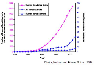
Source: Glazier, Anne M., et al. "Finding Genes that Underlie Complex Traits." *Science* 298, no. 5602 (2002): 2345-9.

Figure 30.5: Discovery of genes for different disease types versus time

only in this context, but also in the contexts of haplotype inference or phasing (assigning alleles to homologous chromosomes) and genotype imputation (inferring missing genotypes based on known genotypes). There have been many optimizations to make this analysis more tractable in practice [1, 11, 12, 15–18, 21, 23].

Linkage analysis identifies a broad genomic region which correlates with the trait of interest. To narrow down the region, we can use fine-resolution genetic maps of recombination breakpoints. We can then identify the affected gene and causal mutation by sequencing the region and testing for altered function.