29.5: Human Evolution

Not surprisingly, the scientific community has a long, and somewhat controversial history of interest in recent population dynamics. While indeed some of this interest was applied toward more nefarious aims, such as the scientific justifications for racism for eugenics but these are increasingly the exception and not the rule. Early studies of population dynamic were primitive in many ways. Quantifying the differences between human populations was originally performed using blood types, as they seemed to be phenotypically neutral, could be tested for outside of the body, and seemed to be polymorphic in many different human populations. Fast forward to the present, and the scientific community has realized that there are other glycoproteins beyond the A,B and O blood groups that are far more polymorphic in the population. As science continued to advance and sequencing became a reality, they began whole genome sequencing of the Y-chromosome, mitochondrial and microsatellite markers around them. What’s special about those two types of genetic data? First and foremost, they are quite short so they can be sequenced more easily than other chromosomes. Beyond just the size, the reason that the Y and mitochondrial chromosomes were of such interest is because they do not recombine, and can be used to easily reconstruct inheritance trees. This is precisely what makes these chromosomes special relative to a short chunk on an autosome; we know exactly where it comes from because we can trace paternal or maternal lineage backward in time.

This type of reconstruction does not work with other chromosomes. If one were to generate a tree using a certain chunk of all of chromosome 1 in a certain population, for instance, they would indeed form a phylogeny but that phylogeny would be picked from random ancestors in each of the family trees.

As sequencing continued to develop and grow more effective, the human genome project was being proposed, and along with it there was a strong push to include some sort of diversity measure in genomic data. Technically speaking, it was easiest to simply look at microsatellites for this diversity measure because they can be studied on gel to see size polymorphisms instead of inspecting a sequence polymorphism. As a reminder, a microsatellite is a region of variable length in the human genome often characterised by short tandem repeats. One reason for microsatellites is retroviruses inserting themselves into the genome, such as the ALU elements in the human genome. These elements sometimes become active and will retro-transpose as insertion events and one can trace when those insertion events have happened in human lineage. Hence, there was a push, early on to assay these parts of the genome in a variety of different populations. The really attractive thing about microsatellites is that they are highly polymorphic and one can actually infer their rate of mutation. Hence, we can not only say that there is a certain relationship between populations based on these rates, but we can also say how long they have been evolving and even when certain mutations occurred, and how long it’s been on certain branches of the phylogenetic tree.

FAQ

Q: Can’t this simply be done with SNPs

A: You can’t do it very easily with SNPs.

You can get an idea of how old they are based on their allele frequency, but they’re also going to be influenced by selection.

After the human genome project, came the Haplotype inheritance Hapmap project which looked at SNPs genome wide. We have discussed Haplotype inheritance in detail in prior chapters where we learned the importance of Hapmap in designing genotyping arrays which look at SNPs that mark common haplotypes in the population.

The effects of Bottlenecks on Human diversity Using this wealth of data across studies and a plethora of mathematical techniques has led to the realization that humans, in fact, have a very low diversity given our census population; which implies a small effective population size. Utilizing the Wright-Fisher model it is possible to work back from the level of diversity and the number of mutations we see in the population today to generate a founding population size. When this computation is performed it works out to being around 10,000.

FAQ

Q: Why is this so much smaller than our census population size?

A: There was A population bottleneck somewhere.

Figure 30.10: A depiction of two major bottleneck events, one in the founding population from Africa, and other, smaller subsequent bottleneck events in the East Asian and Western European populations.

Most of the total variation between humans is happening within-continent. One can measure how much diversity is explained by geography and how much is not. It turns out that most of it is not explained by geography. In fact, most common variants are polymorphic in every population and if a common variant is unique to a given population, there probably hasn’t been enough time for that to happen by drift itself. Recall what an unlikely process it is to get to a high allele frequency over the course of several generations by mere chance alone. Hence, we may interpret this as a signal of selection when it occurs. All of the evidence in terms of comparing diversity patterns and trees back to ancestral haplotypes converges to an Out-of-Africa hypothesis which is the overwhelming consensus in the field and is the lens through which we review all the genetic population data. Starting from the African founder population, there have been works which have demonstrated that it’s possible to model population growth using the wright fisher model. The studies have shown that the growth rate we see in Asian and European populations are only consistent with large exponential growth after the out-of-Africa event.

Table 30.2: Genetic Estimates of Recent Population Growth in Europe

This helps us understand the reasons for phonotypical differences between the races as Bottlenecks which are followed by exponential growth can lead to an excess of rare alleles. The present theory on human diversity states that there were secondary bottleneck events after the founding population migrated out of Africa. These founders were, at some earlier point subject to an even smaller bottleneck event which is now reflected in every human genome on the planet, regardless of their immediate ancestry. It is possible to estimate how small the original bottle neck was by looking at differences between African and European origin individuals, inferring the effects of the secondary bottleneck, and the term of exponential growth of the European population. The other way of approaching bottleneck event estimation is to simply inspect the allele frequency spectrum needed to build coalescent trees. In this way, one can take haplotypes across the genome and ask what the most recent common ancestor was by observing how the coalescence varies across the genome. For instance, one may guess that some haplotype was positively selected for only recently given the length of the haplotype. An example of one such recent mutation in the European population is the lactase gene. Another example for the Asian population is the ER locus.

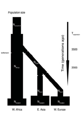
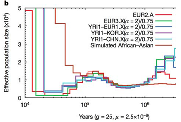
There is a wealth of literature showing that when one draws a coalescence tree for most haplotypes it ends up going way back before when we think speciation happened. This indicates that certain features have been kept polymorphic for a very long time. One can, however, look at this distribution of features across the whole genome and infer something about population history from it. If there was a recent bottle neck in a population, it will be reflected by the ancestors being very recent whereas more ancient things will have survived the bottleneck. One can take the distribution of coalescent times and run simulations for how the effect of population size would have varied with time. The model for doing this type of study was outlined by Li and Durbin. The Figure 29.11 from their study illustrates two such bottleneck events. The first is the bottleneck which occurred in Africa long before migrations out of the continent. This was then followed by a population specific bottleneck that resulted from migration groups out of Africa. This is reflected in the diversity of the populations today based on their ancestry and it can be derived from looking at a pair of chromosome from any two people in these populations.

Figure 29.11: An illustration of two bottleneck events

Understanding Disease

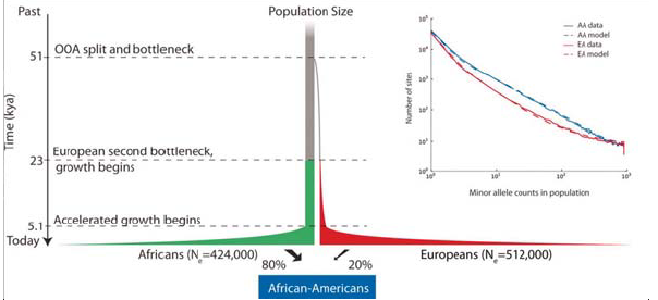
Understanding that human populations went through bottlenecks has important implications for under- standing population specific disease. A study published by Tennessen et al. this year was looking at exome sequences in many classes of individuals. The study intended to look at how rare variants might be contributing to disease and as a consequence they were able to fit population genetics models to the data, and ask what sort of deleterious variants were seen when sequencing exomes from a broad population panel. Using this approach, they were then able to generate parameters which describe how long ago exponential growth between the founder, and branching populations occured. See figure 29.12 below for an illustration of this:

Figure 29.12: The figure illustrate the effects of a bottleneck events on the number of rare Alleles in a population.

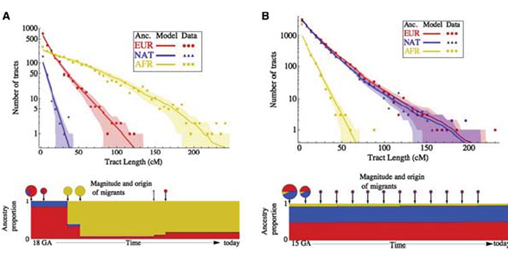
Understanding Recent Population Admixture

In addition to viewing coalescent times, one can also perform Principal Component Analysis on SNPs to gain an understanding of more recent population admixtures. Running this on most populations shows clustering with respect to geographical location. There are some populations, however, that experienced a recent admixture for historical reason. The two most commonly referred to in the scientific literature are: African Americans, who on average are 20

Figure 29.13: A depiction of European admixture levels in the Mexican, and African American populations.

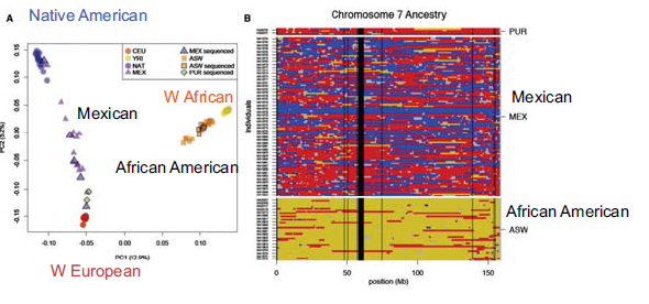
There are two major things one can say about the admixture event of African Americans and Mexican Americans. The first and more obvious is inferring the admixture level. The second, and more interesting, is inferring when the admixture event happened based on the actual mixture level. As we have discussed in previous chapters, the racial signifiers of the genome break down with admixture because of recombination in each generation. If the population is contained, the percentage of those with European and West African origin should stay the same in each generation, but the segments will get shorter, due to the mixing. Hence, the length of the haplotype blocks can be used to date back to when the mixing originally happened. (When it originally happened we would expect large chunks, with some gambits being entirely of African origin, for instance.) Using this approach, one can look at the distribution of recent ancestry traps and then fit a model to when these migrants entered an ancestral population as shown below:

Figure 29.14: As illustration of the magnitude and origin of migrants based on the tract length and number of tracts in the admixed population.