
29.2: Population Selection Basics
- Page ID
- 41135
Polymorphisms
Polymorphisms are differences in appearance amongst members of the same species. Many of them arise from mutations in the genome. These mutations, or genetic polymorphisms, can be characterized into different types.
Single Nucleotide Polymorphisms (SNPs)
• The mutation of only a single nucleotide base within a sequence. In most cases, these changes are without consequence. However, there are some cases where the mutation of a single nucleotide has a major effect.
• For example, is caused by a from A to T, that causes a change from glutamic acid (GAG) to valine (GTG) in hemoglobin.
Variable Number Tandem Repeats
- When a short sequence is repeated multiple times, DNA Polymerase can sometimes ”slip”, causing it to make either too many or too few copies of the repeat. This is called a .
- For example, Huntingtons disease that is caused by too many repeats of the trinucleotide CAG repeat in the HTT gene. Having more than 36 repeats can lead to gradual muscle control loss and severe neurological degradation. Generally, the more repeats there are, the stronger the symptoms.
Insertion/Deletion
- Through faulty copying or DNA-repair, or of one or multiple nucleotides can occur.
- If the insertion or deletion is inside an exon (the protein-coding region of a gene) and does not consist of a multiple of three nucleotides, a will occur.
- Prime example is deletions in the CFTR gene, which codes for chloride channels in the lungs and may cause Cystic Fibrosis where the patient cannot clear mucous in the lungs and causes infection
Did You Know?
DNA profiling is based on short variable number tandem repeats (STR). DNA is cut with certain restriction enzymes, resulting in fragments of variable length that can be used to identify an individual. Different countries use different (but often overlapping) loci for these profiles. In North America, a system based on 13 loci is used.
Allele and Genotype Frequencies
In order to understand the evolution of a species through analysis of alleles or genotypes, we must have a model of how the alleles are passed on from one generation to another. It is of immense importance that the reader has a firm intuition for the Hardy-Weinberg Principle and Wright fisher model before continuing. Hence, we will provide here a short reminder of modelling the history of mutations via the these methods. First introduced over a hundred years ago, the Wright-Fisher Model is a mathematical model of genetic drift in a population. Specifically, it describes the probability of obtaining k copies of a new allele p within a population of size N, with a non-mutant frequency of q, and what its expected frequency will be in successive generations.
Hardy-Weinberg Principle
The states that allele and genotype frequencies within a population will remain constant unless there is an outside influence that pushes them away from that equilibrium.
The Hardy-Weinberg principle is based on the following assumptions:
• The population observed is very large
- The population is isolated, i.e. there is no introduction of another subpopulation into the general population
- All individuals have equal probability of producing offspring
- All mating in the population is at random
- No random mutations occur in the population from one generation to the next
- Allele frequency drives future genotype frequency (Prevalent allele drives Prevalent genotype)
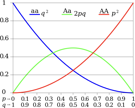
In a Hardy-Weinberg Equilibrium, for two alleles A and a, occurring with probability p and q = 1p, respectively, the probabilities of a randomly chosen individual having the homozygous AA or aa (pp or qq, respectively) or heterozygous Aa or aA (2pq) genotypes can be described by the equation:
\[p^{2}|2 p q| q^{2}=1\nonumber\]
This equation gives a table of probabilities for each genotype, which can be compared with the observed genotype frequencies using statistical error tests such as the chi-squared test to determine if the Hardy- Weinberg model is applicable. Figure 29.1 shows the distribution of genotype frequencies at different allele frequencies.
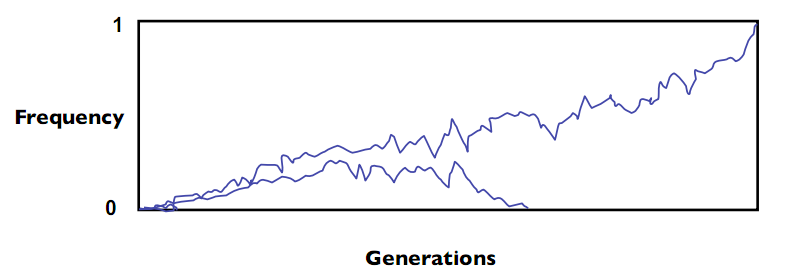
In natural populations, the assumptions made by the Hardy-Weinberg principle will rarely hold. Natural selection occurs, small populations undergo genetic drift, populations are split or merged, etc. In Nature a mutation will always either disappear (frequency = 0) from the population or become prevalent in a species - this is called fixation; in general, 99% of mutations disappear. Figure 29.2 shows a simulation of a mutations prevalence in a finite-sized population over time: both perform random walks, with one mutation disappearing and the other becoming prevalent:
Once a mutation has disappeared, the only way for it to reappear is the introduction of a new mutation into the population. For humans, it is believed that a given mutation under no selective pressure should fixate to 0 or 1 (within, e.g., 5%) within a few million years. However, under selection this will happen much faster.
Wright-Fisher Model
Under this model the time to fixation is 4N and the probability of fixation is 1/2N. In general Wright-Fisher is used to answer questions related to fixation in one way or another. To make sure your intuitions about
Commons license. For more information, see http://ocw.mit.edu/help/faq-fair-use/.
Figure 29.2 Changes in allele frequency over time.
the method are absolutely clear considering the following questions:
FAQ
Q: Say you have a total of 5 mutations on a chromosome among a population of size 30, on average, how many mutations will be present in the next generation if each entity produces only one child?
A: If each parent has only one offspring, then there will be, on average, 5 mutations in the next generation because the expectation of allele frequencies is to remain constant according to the Hardy-Weinberg equilibrium principle in basic biology.
FAQ
Q: Is the Hardy-Weinberg Equilibrium principle’s assumption about constant allele frequency reasonable?
A: No, the reality is far more complex as there is stochasticity in population size and selection at each generation. A more appropriate way to envision this is to image drawing alleles from a set of parents, with the amount of alleles in the next generation varying with the size of the population. Hence the frequency in the next generation could very well go up or down. Note here that if the allele frequency goes to zero it will always be at zero. The probability at each successive generation is lower if it’s under negative selection and higher if it’s under positive selection. Hence if it’s a beneficial mutation the fixation time will be smaller, if the mutation is deleterious the fixation will be larger. If there are no offspring with a given mutation, then there won’t be any decedents with that mutation either. If one produces multiple o↵spring however, who in turn produce multiple offspring of their own, then there is a greater chance that this allele frequency will rise.
FAQ
Q: Consider that the average human individual carries roughly 100 entirely unique mutations. So, when an individual produces offspring we could expect that half (or 50) of those mutations may appear in the child because in each sperm or egg cell, 50 of those mutations will be present, on average. Hence the offspring of an individual are likely to inherit approximately 100 mutations, 50 from one parent, and 50 from another in addition to their own unique mutations which come from neither parent. With this in mind, one might be interested in understanding what the chances are of some mutations appearing in the next generation if an individual produces, say, n children. How can one do this?
A: Hint: To compute this value, we assume that some allele originates in the founder, at some arbitrary chromosome (1 for example). Then we ask the question, how many chromosome 1s exist in the entire population? At the moment, the size of the human population is 7 Billion, each carrying two copies of chromosome 1.
The above questions and answers should make it painfully clear that the standard Hardy-Weinberg assumption of allele frequencies remaining constant from one generation to the next is violated in many natural cases including migration, genetic mutation, and selection. In the case of selection, this issue is addressed by modifying the formal definition to include a S, term which measures the skew in genotypes due to selection. See table 29.1 for a comparison of the original and selection compensated versions:
| Behavior | With only drift | With drift and selection |
| n in next generation | Mean: n(=2Np), Dist: Binomial(2N, p) | Mean: n(\(n\left(1+\frac{s}{1+n s}\right)\)), Dist: Binomial(2N, \(2 N, p \frac{1+s}{1+p s}\)) |
| Time to fixation | 4N | \(\frac{4 N}{1+\frac{3}{4} N|s|}\left(\frac{1+\frac{1}{2}(\ln N)|s|}{1+|s|}\right)\) |
| Probability of fixation | \(\frac{1}{2 N}\) | \(\frac{1-e^{-2 a}}{1-e^{-4 N s}}\) |
Table 29.1: Comparison of Wright-Fisher Model With Drift, Versus Drift and Selection
The main point to take away from Table 29.1, and this section of the chapter is that weather you have selection or not, it is highly unlikely that a single allele will fixate in a population. If you have a very small population, however, then the chances of an allele fixating are much better. This is often the case in human populations, where there are often small, interbred populations which allow for mutations to fix in a population after only a few generations, even if the mutation is deleterious in nature. This is precisely why we tend to see recessive deleterious mandolin disorders in isolated populations.
Ancestral State of Polymorphisms
How can we determine for a given polymorphism which version was the and which one is the mutant? The ancestral state can be inferred by comparing the genome to that of a closely related species (e.g. humans and chimpanzees) with a known phylogenetic tree. Mutations can occur anywhere along the phylogenetic tree sometimes mutations at the split fix differently in different populations (“fixed difference”), in which case the entire populations differ in genotype. However, recent mutations will not have had enough time to become fixed, and a polymorphism will be present in one species but fully absent in the other as simultaneous mutations in both species are very rare. In this case, the “derived variant” is the version of the polymorphism appearing after the split, while the ancestral variant is the version occuring in both species.
Commons license. For more information, see http://ocw.mit.edu/help/faq-fair-use/.
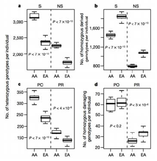
Figure 30.3: A comparison of the hetrozygous and homozygous derived and damaging genotypes per individual in an African American (AA) and European American (EA) population study.
29.2.4 Measuring Derived Allele Frequencies
The the frequency of the derived allele in the population can be easily calculated, if we assume that the population is homogeneous. However, this assumption may not hold when there is an unseen divide between two groups that causes them to evolve separately as shown in figure 29.4.
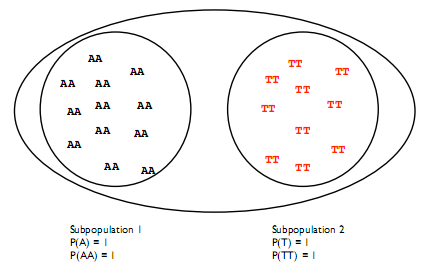
In this case the prevalence of the variants among subpopulations is different and the Hardy-Weinberg principle is violated.
One way to quantify this difference is to use the (Fst) to compare subpopulations within a species. In reality only a portion of the total heterozygosity in a species is found in a given subpopulation. Fst estimates the reduction in heterozygosity (2pq with alleles p and q) expected when 2 different populations are erroneously grouped together. Given a population having n alleles with frequencies pi where \((1 \leq i \leq n)\), the homozygosity G of the population is calculated as:
\[\Sigma_{i=1}^{n} p_{i}^{2}\nonumber\]
The total heterozygosity in the population is given by 1-G.
\[F_{s t}=\frac{H \text {eterozygosity}(\text {total})-\text {Heterozygosity}(\text {subpopulation})}{\text {Heterozygosity}(\text {total})}\nonumber\]
In the case shown in figure 29.4 there is no heterozygosity between the populations, so Fst = 1. In reality the Fst will be small within one species. In humans, for example, it is only 0.0625. For in practise, the Fst is computed either by clustering sub-populations randomly or using an obvious characteristic such as ethnicity or origin.