28.8: European Ancestry and Migrations

Tracing the Origins of European Genetics

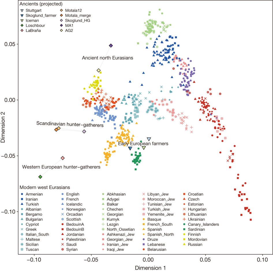
Before 2014, it was believed that modern European genetics was primarily a mixture of two ancestral populations. The first population is what is known as the Western hunter-gathere (WHG) population, and is considered the indigenous European population. The second population is known as the Early European farmer (EEF) population, and represents the rapid migration of farming peoples into Europe, and the subsequent mixing of the new farming population with the original WHG population. However, in 2012, Patterson et al [? ] used the principal component analysis in Figure 29.6 to show that European genetics does not match up with being a mixture of only these two populations. Rather, genetic mixture analysis showed that some Europeans could only be explained as a mix of EEF/WHG populations with a third population whose genetics resembled Native Americans. While this does not mean that Native Americans are ancestral to Europeans, the study concluded that the most likely hypothesis was the mixture of these two known populations with an Ancient North Eurasian (ANE) population which migrated to both Asia and Europe, and is no longer found in North Eurasia. This study called this mystery population the ”Ghost of North Eurasia.”

Two years later, in 2014, however, a sample was found confirming the existence of this population. Proclaiming that ”The ghost is Found”, Raghavan, Skoglund et al. [? ] studied the newly found ”Mal’ta” sample from Lake Baikal (currently in Southern Russia) and determined that it matched the predicted ghost population from 2012, and could explain the two dimensional variation in modern European populations. In particular, modern Europeans were found to be composed of 0-50% WHG, 32-93% EEF, and 1-18% ANE populations.

Migration from the Steppe

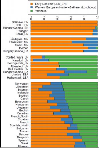
Given this new population as a source of European ancestry, the natural questions are when and why did the members of the ANE population migrate to Europe? The answer, of course, can be teased out of further genetic data about the history of European populations. The first clue was found in mitochondrial DNA data, in a 2013 paper by Brandt, Haak et al. [? ], which found that there were two discontinuities in European mitochondrial DNA: one between the Mesolithic and the early Neolithic ages, and one between the mid Neolithic age and the Late Neolithic and Bronze ages. In 2014, studies of 9, and then 94 samples of ancient European individuals showed clearly the two migration events, visualized in Figure 29.7. The first migration, at roughly 6500 BCE, was a migration of the EEF population, which replaced the existing WHG population at a rate of between 60 and 100%. The second migration was a migration of steppe pastoralists, known as the Yamnaya, which replaced the existing population with a rate between 60 and 80%. In both

Courtesy of Macmilan Publishers Limited. Used with permission.

Source: Lazaridis, Iosif, et al. "Ancient Human Genomes Suggest Three Ancestral

Populations for Present-day Europeans." Nature 513, no. 7518 (2014): 409-13

Figure 28.6: Ancient Europeans projected onto the two dimensional PCP of all modern European populations. The modern Western Europeans, represented primarily by the bottom left cline, cannot be described as a mixture of only EEF and WHG populations. However, with the addition of an ANE component, the variations can be explained.

cases, the migrating population takes over a chunk of the genetic composition almost immediately, and then the previous population gradually resurges over several thousand years.

Screening for Natural Selection

Another application of DNA data to history is in tracing natural selection events. Essentially, one can look at the frequencies of various alleles in modern European DNA data, and find cases where it does not match the ancestral mixing model of the population. Such cases will tend to signify alleles that have been selected for or against since the ancestral mixing events occurred. The easiest to identify, and most well known example of such a trait is lactase persistence. The current level of prevalence of this trait is well above any of the levels represented by ancestral populations, suggesting that it underwent positive selection (due to the domestication and milking of animals) since the ancestral mixing events.

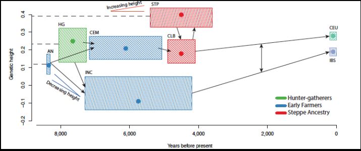
Several other traits can also be detected as candidates for selection. Another straightforward example is skin pigmentation. More interesting is the tale of height selection shown by the genetics of Northern and Southern Europeans. In particular, the data shows that two distinct selection effects occurred. First, the early farmers of Southern Europe underwent selection for decreasing height between 8000 and 4000 years ago. Second, the peoples of Northern Europe (modern Scandinavians, etc.) underwent positive selection around the same time period and through the present. While the anthropological explanations of these effects are disputed, the effects themselves are shown clearly in the genetic data.

Courtesy of Macmilan Publishers Limited. Used with permission.

Source: Haak, Wolfgang, et al. "Massive Migration from the Steppe

was a Source for Indo-European Languages in Europe." Nature (2015).

Figure 29.7: European genetic composition over time shows two massive migrations: first, the migration of the EEF population, almost completely replacing the native WHG population; and second, the migration of the ANE Yamnaya population, replacing about 75% of the native population at that point.

Figure 28.8: Height selection in European populations from 8000 years ago to the present.

Courtesy of Macmilan Publishers Limited. Used with permission.

Source: Mathieson, Iain et al. "Genome-wide Patterns of Selection

in 230 Ancient Eurasians." Nature 528, no. 7583 (2015): 499-503.