27.2: SPIDR
- Page ID
- 41074
\( \newcommand{\vecs}[1]{\overset { \scriptstyle \rightharpoonup} {\mathbf{#1}} } \)
\( \newcommand{\vecd}[1]{\overset{-\!-\!\rightharpoonup}{\vphantom{a}\smash {#1}}} \)
\( \newcommand{\id}{\mathrm{id}}\) \( \newcommand{\Span}{\mathrm{span}}\)
( \newcommand{\kernel}{\mathrm{null}\,}\) \( \newcommand{\range}{\mathrm{range}\,}\)
\( \newcommand{\RealPart}{\mathrm{Re}}\) \( \newcommand{\ImaginaryPart}{\mathrm{Im}}\)
\( \newcommand{\Argument}{\mathrm{Arg}}\) \( \newcommand{\norm}[1]{\| #1 \|}\)
\( \newcommand{\inner}[2]{\langle #1, #2 \rangle}\)
\( \newcommand{\Span}{\mathrm{span}}\)
\( \newcommand{\id}{\mathrm{id}}\)
\( \newcommand{\Span}{\mathrm{span}}\)
\( \newcommand{\kernel}{\mathrm{null}\,}\)
\( \newcommand{\range}{\mathrm{range}\,}\)
\( \newcommand{\RealPart}{\mathrm{Re}}\)
\( \newcommand{\ImaginaryPart}{\mathrm{Im}}\)
\( \newcommand{\Argument}{\mathrm{Arg}}\)
\( \newcommand{\norm}[1]{\| #1 \|}\)
\( \newcommand{\inner}[2]{\langle #1, #2 \rangle}\)
\( \newcommand{\Span}{\mathrm{span}}\) \( \newcommand{\AA}{\unicode[.8,0]{x212B}}\)
\( \newcommand{\vectorA}[1]{\vec{#1}} % arrow\)
\( \newcommand{\vectorAt}[1]{\vec{\text{#1}}} % arrow\)
\( \newcommand{\vectorB}[1]{\overset { \scriptstyle \rightharpoonup} {\mathbf{#1}} } \)
\( \newcommand{\vectorC}[1]{\textbf{#1}} \)
\( \newcommand{\vectorD}[1]{\overrightarrow{#1}} \)
\( \newcommand{\vectorDt}[1]{\overrightarrow{\text{#1}}} \)
\( \newcommand{\vectE}[1]{\overset{-\!-\!\rightharpoonup}{\vphantom{a}\smash{\mathbf {#1}}}} \)
\( \newcommand{\vecs}[1]{\overset { \scriptstyle \rightharpoonup} {\mathbf{#1}} } \)
\( \newcommand{\vecd}[1]{\overset{-\!-\!\rightharpoonup}{\vphantom{a}\smash {#1}}} \)
\(\newcommand{\avec}{\mathbf a}\) \(\newcommand{\bvec}{\mathbf b}\) \(\newcommand{\cvec}{\mathbf c}\) \(\newcommand{\dvec}{\mathbf d}\) \(\newcommand{\dtil}{\widetilde{\mathbf d}}\) \(\newcommand{\evec}{\mathbf e}\) \(\newcommand{\fvec}{\mathbf f}\) \(\newcommand{\nvec}{\mathbf n}\) \(\newcommand{\pvec}{\mathbf p}\) \(\newcommand{\qvec}{\mathbf q}\) \(\newcommand{\svec}{\mathbf s}\) \(\newcommand{\tvec}{\mathbf t}\) \(\newcommand{\uvec}{\mathbf u}\) \(\newcommand{\vvec}{\mathbf v}\) \(\newcommand{\wvec}{\mathbf w}\) \(\newcommand{\xvec}{\mathbf x}\) \(\newcommand{\yvec}{\mathbf y}\) \(\newcommand{\zvec}{\mathbf z}\) \(\newcommand{\rvec}{\mathbf r}\) \(\newcommand{\mvec}{\mathbf m}\) \(\newcommand{\zerovec}{\mathbf 0}\) \(\newcommand{\onevec}{\mathbf 1}\) \(\newcommand{\real}{\mathbb R}\) \(\newcommand{\twovec}[2]{\left[\begin{array}{r}#1 \\ #2 \end{array}\right]}\) \(\newcommand{\ctwovec}[2]{\left[\begin{array}{c}#1 \\ #2 \end{array}\right]}\) \(\newcommand{\threevec}[3]{\left[\begin{array}{r}#1 \\ #2 \\ #3 \end{array}\right]}\) \(\newcommand{\cthreevec}[3]{\left[\begin{array}{c}#1 \\ #2 \\ #3 \end{array}\right]}\) \(\newcommand{\fourvec}[4]{\left[\begin{array}{r}#1 \\ #2 \\ #3 \\ #4 \end{array}\right]}\) \(\newcommand{\cfourvec}[4]{\left[\begin{array}{c}#1 \\ #2 \\ #3 \\ #4 \end{array}\right]}\) \(\newcommand{\fivevec}[5]{\left[\begin{array}{r}#1 \\ #2 \\ #3 \\ #4 \\ #5 \\ \end{array}\right]}\) \(\newcommand{\cfivevec}[5]{\left[\begin{array}{c}#1 \\ #2 \\ #3 \\ #4 \\ #5 \\ \end{array}\right]}\) \(\newcommand{\mattwo}[4]{\left[\begin{array}{rr}#1 \amp #2 \\ #3 \amp #4 \\ \end{array}\right]}\) \(\newcommand{\laspan}[1]{\text{Span}\{#1\}}\) \(\newcommand{\bcal}{\cal B}\) \(\newcommand{\ccal}{\cal C}\) \(\newcommand{\scal}{\cal S}\) \(\newcommand{\wcal}{\cal W}\) \(\newcommand{\ecal}{\cal E}\) \(\newcommand{\coords}[2]{\left\{#1\right\}_{#2}}\) \(\newcommand{\gray}[1]{\color{gray}{#1}}\) \(\newcommand{\lgray}[1]{\color{lightgray}{#1}}\) \(\newcommand{\rank}{\operatorname{rank}}\) \(\newcommand{\row}{\text{Row}}\) \(\newcommand{\col}{\text{Col}}\) \(\renewcommand{\row}{\text{Row}}\) \(\newcommand{\nul}{\text{Nul}}\) \(\newcommand{\var}{\text{Var}}\) \(\newcommand{\corr}{\text{corr}}\) \(\newcommand{\len}[1]{\left|#1\right|}\) \(\newcommand{\bbar}{\overline{\bvec}}\) \(\newcommand{\bhat}{\widehat{\bvec}}\) \(\newcommand{\bperp}{\bvec^\perp}\) \(\newcommand{\xhat}{\widehat{\xvec}}\) \(\newcommand{\vhat}{\widehat{\vvec}}\) \(\newcommand{\uhat}{\widehat{\uvec}}\) \(\newcommand{\what}{\widehat{\wvec}}\) \(\newcommand{\Sighat}{\widehat{\Sigma}}\) \(\newcommand{\lt}{<}\) \(\newcommand{\gt}{>}\) \(\newcommand{\amp}{&}\) \(\definecolor{fillinmathshade}{gray}{0.9}\)Background
As presented in the supplementary information for SPIDIR, a gene family is the set of genes that are descendents of a single gene in the most recent common ancestor (MRCA) of all species under consideration. Furthermore, genetic sequences undergo evolution at multiple scales, namely at the level of base pairs, and at the level of genes. In the context of this lecture, two genes are orthologs if their MRCA is a speciation event; two genes are paralogs if their MRCA is a duplication event.
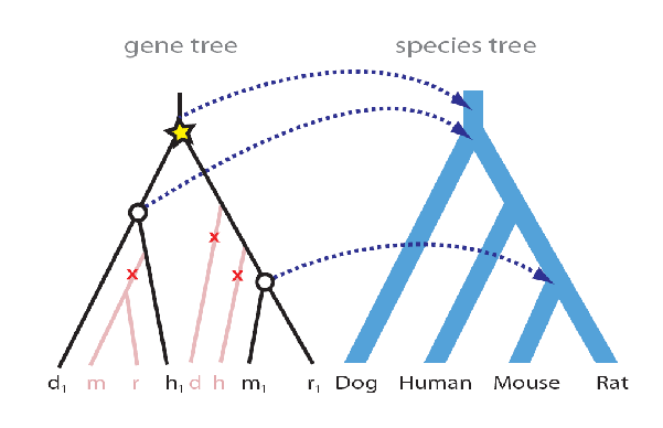
In the genomic era, the species of a modern genes is often known; ancestral genes can be inferred by reconciling gene- and species-trees. A reconciliation maps every gene-tree node to a species-tree node. A common technique is to perform Maximum Parsimony Reconciliation (MPR), which finds the reconciliation R implying the fewest number of duplications or losses using the recursion over inner nodes v of a gene tree G. MPR fist maps each leaf of the gene tree to the corresponding species leaf of the species tree. Then the internal nodes of G are mapped recursively:
\[R(v)=\operatorname{MRCA}(R(\operatorname{right}(v)), R(\operatorname{left}(v)))\nonumber\]
If a speciation event and its ancestral node are mapped to the same node on the species tree. Then the ancestral node must be an duplication event.Using MPR, the accuracy of the gene tree is crucial. Suboptimal gene trees may lead to an excess of loss and duplication events. For example, if just one branch is misplaced (as in ??) then reconciliation infers 3 losses and 1 duplication event. In [6], the authors show that the contemporaneous current gene tree methods perform poorly (60% accuracy) on single genes. But if we have longer concatenated genes, then accuracy may go up towards 100%. Furthermore, very quickly or slowly evolving genes carry less information as compared with moderately diverging sequences (40-50% sequence identity), and perform correspondingly worse. As corroborated by simulations, single genes lack sucient information to reproduce the correct species tree. Average genes are too short and contains too few phylogenetically informative characters. While many early gene tree construction algorithms ignored species information, algorithms like SPIDIR capitalize on the insight that the species tree can provide additional information which can be leveraged for gene tree construction. Synteny can be used to independently test the relative accuracy of di↵erent gene tree reconstructions. This is because syntenic blocks are regions of the genome where recently diverged organisms have the same gene order, and contain much more information than single genes.


There have been a number of recent phylogenomic algorithms including: RIO [2], which uses neighbor joining (NJ) and bootstrapping to deal with incogruencies, Orthostrapper [7], which uses NJ and reconciles to a vague species tree, TreeFAM [3], which uses human curation of gene trees as well as many others. A number of algorithms take a more similar track to SPIDIR [6], including [4], a probabilistic reconciliation algorithm [8], a Bayesian method with a clock,[9],and parsimony method using species tree , as well as more recent developments: [1] a Bayesian method with relaxed clock and [5], a Bayesian method with gene and species specific relaxed rates (an extension to SPIDIR) .
Method and Model
SPIDIR exemplifies an iterative algorithm for gene tree construction using the species tree. In SPIDIR, the authors define a generative model for gene-tree evolution. This consists of a prior for gene-tree topology and branch lengths. SPIDIR uses a birth and death process to model duplications and losses (which informs the prior on topology) and then then learns gene-specific and species-specific substitution rates (which inform the prior on branch lengths). SPIDIR is a Maximum a posteriori (MAP) method, and, as such, enjoys several nice optimality criteria.
In terms of the estimation problem, the full SPIDIR model appears as follows:
\[\operatorname{argmax} L, T, R P(L, T, R \mid D, S, \Theta)=\operatorname{argmax} L, T, R P(D \mid T, L) P(L \mid T, R, S, \Theta) P(T, R \mid S, \Theta)\nonumber\]
The parameters in the above equation are: D = alignment data , L = branch length T = gene tree topology , R = reconciliation , S = species tree (expressed in times) , \(\Theta\) = ( gene and species specific parameters [estimated using EM training], , μ dup/loss parameters)). This model can be understood through the three terms in the right hand expression, namely:
- the sequence model– P(D|T,L). The authors used the common HKY model for sequence substitutions, which unifies Kimura’s two parameter model for transitions and transversions with Felsenstein’s model where substitution rate depends upon nucleotide equilibrium frequency.
- the first prior term, for the rates model– P(L|T,R,S,\(\Theta\)), which the authors compute numerically after learning species and gene specific rates.
- the second prior term, for the duplication/loss model– P(T,R|S,\(\Theta\)), which the authors describe using a birth and death process.
Having a rates model is very rates model very useful, since mutation rates are quite variable across genes. In the lecture, we saw how rates were well described by a decomposition into gene and species specific rates. In lecture we saw that an inverse gamma distribution appears to parametrize the gene specific substitution rates, and we were told that a gamma distribution apparently captures species specific substitution rates. Accounting for gene and species specific rates allows SPIDIR to build gene trees more accurately than previous methods. A training set for learning rate parameters can be chosen from gene trees which are congruent to the species tree. An important algorithmic concern for gene tree reconstructions is devising a fast tree search method. In lecture, we saw how the tree search could be sped up by only computing the full argmaxL,T,RP(L,T,R|D,S,\(\Theta\)) for trees with high prior probabilites. This is accomplished through a computational pipeline where in each iteration 100s of trees are proposed by some heuristic. The topology prior P(T,R|D,S,\(\Theta\)) can be computed quickly. This is used as a filter where only the topologies with high prior probabilities are selected as candidates for the full likelihood computation.
The performance of SPIDIR was tested on a real dataset of 21 fungi. SPIDER recovered over 96% of the synteny orthologs while other algorithms found less than 65%. As a result, SPIDER invoked much fewer number of duplications and losses.

