18.1: Introduction to Regulatory Genomics

Last updated
Save as PDF

Page ID: 41023

\( \newcommand{\vecs}[1]{\overset { \scriptstyle \rightharpoonup} {\mathbf{#1}} } \) \( \newcommand{\vecd}[1]{\overset{-\!-\!\rightharpoonup}{\vphantom{a}\smash {#1}}} \)\(\newcommand{\id}{\mathrm{id}}\) \( \newcommand{\Span}{\mathrm{span}}\) \( \newcommand{\kernel}{\mathrm{null}\,}\) \( \newcommand{\range}{\mathrm{range}\,}\) \( \newcommand{\RealPart}{\mathrm{Re}}\) \( \newcommand{\ImaginaryPart}{\mathrm{Im}}\) \( \newcommand{\Argument}{\mathrm{Arg}}\) \( \newcommand{\norm}[1]{\| #1 \|}\) \( \newcommand{\inner}[2]{\langle #1, #2 \rangle}\) \( \newcommand{\Span}{\mathrm{span}}\) \(\newcommand{\id}{\mathrm{id}}\) \( \newcommand{\Span}{\mathrm{span}}\) \( \newcommand{\kernel}{\mathrm{null}\,}\) \( \newcommand{\range}{\mathrm{range}\,}\) \( \newcommand{\RealPart}{\mathrm{Re}}\) \( \newcommand{\ImaginaryPart}{\mathrm{Im}}\) \( \newcommand{\Argument}{\mathrm{Arg}}\) \( \newcommand{\norm}[1]{\| #1 \|}\) \( \newcommand{\inner}[2]{\langle #1, #2 \rangle}\) \( \newcommand{\Span}{\mathrm{span}}\)\(\newcommand{\AA}{\unicode[.8,0]{x212B}}\)

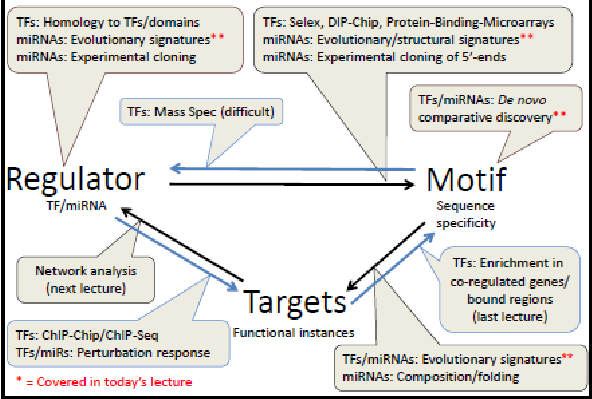
Every cell has the same DNA, but they all have different expression patterns due to the temporal and spatial regulation of genes. Regulatory genomics explains these complex gene expression patterns. The regulators we will be discussing are:

Transcription Factor (TF)- Regulates transcription of DNA to mRNA. TFs are proteins which bind to DNA before transcription and either increase or decrease transcription. We can determine the specificity of a TF through experimental methods using protein or antibodies. We can find the genes by their similarity to know TFs.
Micro RNA (miRNA)- Regulates translation of mRNA to Proteins. miRNAs are RNA molecules which bind to mRNA after transcription and can reduce translation. We can determine the specificity of an miRNA through experimental methods, such as cloning, or computational methods, using conservation and structure.

Open Problems

Both TFs and miRNAs are regulators and we can find them through both experimental and computational methods. We will discuss some of these computational methods, specifically the use of evolutionary signatures. These regulators bind to specific patterns, called motifs. We can predict the motifs to which a regulator will bind using both experimental and computational methods. We will be discussing identification of miRNAs through evolutionary and structural signatures and the identification of both TFs and miRNAs through de novo comparative discovery, which theoretically can find all motifs. Given a motif, it is difficult to find the regulator which binds to it.

A target is a place where a factor binds. There are many sequence motifs, however many will not bind; only a subset will be targets. Targets for a specified regulator can be determined using experimental methods. In Lecture 11, methods for finding a motif given a target were discussed. We will also discuss finding targets given a motif.

Figure 18.1: Challenges in Regulatory Genomics