9.8: Conclusion, Bibliography

Last updated
Save as PDF

Page ID: 40973

\( \newcommand{\vecs}[1]{\overset { \scriptstyle \rightharpoonup} {\mathbf{#1}} } \) \( \newcommand{\vecd}[1]{\overset{-\!-\!\rightharpoonup}{\vphantom{a}\smash {#1}}} \)\(\newcommand{\id}{\mathrm{id}}\) \( \newcommand{\Span}{\mathrm{span}}\) \( \newcommand{\kernel}{\mathrm{null}\,}\) \( \newcommand{\range}{\mathrm{range}\,}\) \( \newcommand{\RealPart}{\mathrm{Re}}\) \( \newcommand{\ImaginaryPart}{\mathrm{Im}}\) \( \newcommand{\Argument}{\mathrm{Arg}}\) \( \newcommand{\norm}[1]{\| #1 \|}\) \( \newcommand{\inner}[2]{\langle #1, #2 \rangle}\) \( \newcommand{\Span}{\mathrm{span}}\) \(\newcommand{\id}{\mathrm{id}}\) \( \newcommand{\Span}{\mathrm{span}}\) \( \newcommand{\kernel}{\mathrm{null}\,}\) \( \newcommand{\range}{\mathrm{range}\,}\) \( \newcommand{\RealPart}{\mathrm{Re}}\) \( \newcommand{\ImaginaryPart}{\mathrm{Im}}\) \( \newcommand{\Argument}{\mathrm{Arg}}\) \( \newcommand{\norm}[1]{\| #1 \|}\) \( \newcommand{\inner}[2]{\langle #1, #2 \rangle}\) \( \newcommand{\Span}{\mathrm{span}}\)\(\newcommand{\AA}{\unicode[.8,0]{x212B}}\)

Computational gene identification, because it entails finding the functional elements encoded within a genome, has a lot of practical significance as well as theoretical significance for the advancement of bio- logical fields.

The two approaches described above are summarized below in Figure 9.11:

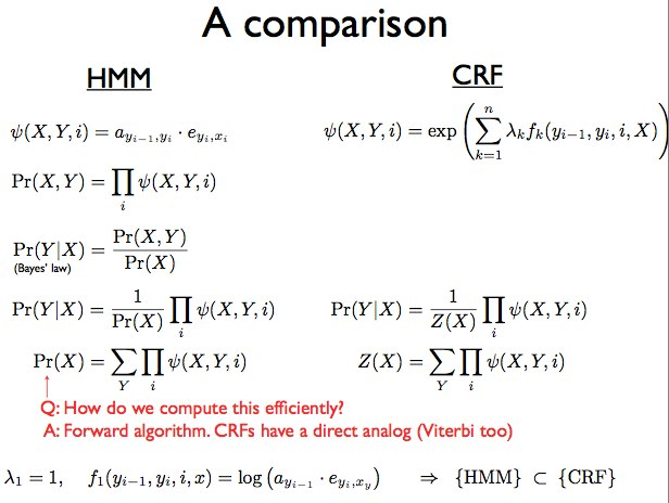
Figure 9.11: A comparison of HMMs and CRFs

HMM

• generative model
• randomly generates observable data, usually with a hidden state
• specifies a joint probability distribution
• P(x,y) = P(x|y)P(y)
• sometimes hard to model dependencies correctly
• hidden states are the labels for each DNA base/letter
• composite emissions are a combination of the DNA base/letter being emitted with additional evidence

CRF

• discriminative model
• models dependence of unobserved variable y on an observed variable x • P(y|x)
• hard to train without supervision
• more effective for when the model doesnt require joint distribution

In practice, the resulting gene specification using CONTRAST, a CRF implementation, is about 46.2% at its maximum. This is because in biology, there are a lot of exceptions to the standard model, such as overlapping genes, nested genes, and alternative splicing. Having models include all of those exceptions sometimes yields worse predictions; this is a non-trivial tradeoff. However, technology is improving and within the next five years, there will be more experimental data to fuel the development of computational gene identification, which in turn will help generate a better understanding of the syntax of DNA.