
36: Western Blot
- Page ID
- 135793

\( \newcommand{\vecs}[1]{\overset { \scriptstyle \rightharpoonup} {\mathbf{#1}} } \)
\( \newcommand{\vecd}[1]{\overset{-\!-\!\rightharpoonup}{\vphantom{a}\smash {#1}}} \)
\( \newcommand{\dsum}{\displaystyle\sum\limits} \)
\( \newcommand{\dint}{\displaystyle\int\limits} \)
\( \newcommand{\dlim}{\displaystyle\lim\limits} \)
\( \newcommand{\id}{\mathrm{id}}\) \( \newcommand{\Span}{\mathrm{span}}\)
( \newcommand{\kernel}{\mathrm{null}\,}\) \( \newcommand{\range}{\mathrm{range}\,}\)
\( \newcommand{\RealPart}{\mathrm{Re}}\) \( \newcommand{\ImaginaryPart}{\mathrm{Im}}\)
\( \newcommand{\Argument}{\mathrm{Arg}}\) \( \newcommand{\norm}[1]{\| #1 \|}\)
\( \newcommand{\inner}[2]{\langle #1, #2 \rangle}\)
\( \newcommand{\Span}{\mathrm{span}}\)
\( \newcommand{\id}{\mathrm{id}}\)
\( \newcommand{\Span}{\mathrm{span}}\)
\( \newcommand{\kernel}{\mathrm{null}\,}\)
\( \newcommand{\range}{\mathrm{range}\,}\)
\( \newcommand{\RealPart}{\mathrm{Re}}\)
\( \newcommand{\ImaginaryPart}{\mathrm{Im}}\)
\( \newcommand{\Argument}{\mathrm{Arg}}\)
\( \newcommand{\norm}[1]{\| #1 \|}\)
\( \newcommand{\inner}[2]{\langle #1, #2 \rangle}\)
\( \newcommand{\Span}{\mathrm{span}}\) \( \newcommand{\AA}{\unicode[.8,0]{x212B}}\)
\( \newcommand{\vectorA}[1]{\vec{#1}} % arrow\)
\( \newcommand{\vectorAt}[1]{\vec{\text{#1}}} % arrow\)
\( \newcommand{\vectorB}[1]{\overset { \scriptstyle \rightharpoonup} {\mathbf{#1}} } \)
\( \newcommand{\vectorC}[1]{\textbf{#1}} \)
\( \newcommand{\vectorD}[1]{\overrightarrow{#1}} \)
\( \newcommand{\vectorDt}[1]{\overrightarrow{\text{#1}}} \)
\( \newcommand{\vectE}[1]{\overset{-\!-\!\rightharpoonup}{\vphantom{a}\smash{\mathbf {#1}}}} \)
\( \newcommand{\vecs}[1]{\overset { \scriptstyle \rightharpoonup} {\mathbf{#1}} } \)
\(\newcommand{\longvect}{\overrightarrow}\)
\( \newcommand{\vecd}[1]{\overset{-\!-\!\rightharpoonup}{\vphantom{a}\smash {#1}}} \)
\(\newcommand{\avec}{\mathbf a}\) \(\newcommand{\bvec}{\mathbf b}\) \(\newcommand{\cvec}{\mathbf c}\) \(\newcommand{\dvec}{\mathbf d}\) \(\newcommand{\dtil}{\widetilde{\mathbf d}}\) \(\newcommand{\evec}{\mathbf e}\) \(\newcommand{\fvec}{\mathbf f}\) \(\newcommand{\nvec}{\mathbf n}\) \(\newcommand{\pvec}{\mathbf p}\) \(\newcommand{\qvec}{\mathbf q}\) \(\newcommand{\svec}{\mathbf s}\) \(\newcommand{\tvec}{\mathbf t}\) \(\newcommand{\uvec}{\mathbf u}\) \(\newcommand{\vvec}{\mathbf v}\) \(\newcommand{\wvec}{\mathbf w}\) \(\newcommand{\xvec}{\mathbf x}\) \(\newcommand{\yvec}{\mathbf y}\) \(\newcommand{\zvec}{\mathbf z}\) \(\newcommand{\rvec}{\mathbf r}\) \(\newcommand{\mvec}{\mathbf m}\) \(\newcommand{\zerovec}{\mathbf 0}\) \(\newcommand{\onevec}{\mathbf 1}\) \(\newcommand{\real}{\mathbb R}\) \(\newcommand{\twovec}[2]{\left[\begin{array}{r}#1 \\ #2 \end{array}\right]}\) \(\newcommand{\ctwovec}[2]{\left[\begin{array}{c}#1 \\ #2 \end{array}\right]}\) \(\newcommand{\threevec}[3]{\left[\begin{array}{r}#1 \\ #2 \\ #3 \end{array}\right]}\) \(\newcommand{\cthreevec}[3]{\left[\begin{array}{c}#1 \\ #2 \\ #3 \end{array}\right]}\) \(\newcommand{\fourvec}[4]{\left[\begin{array}{r}#1 \\ #2 \\ #3 \\ #4 \end{array}\right]}\) \(\newcommand{\cfourvec}[4]{\left[\begin{array}{c}#1 \\ #2 \\ #3 \\ #4 \end{array}\right]}\) \(\newcommand{\fivevec}[5]{\left[\begin{array}{r}#1 \\ #2 \\ #3 \\ #4 \\ #5 \\ \end{array}\right]}\) \(\newcommand{\cfivevec}[5]{\left[\begin{array}{c}#1 \\ #2 \\ #3 \\ #4 \\ #5 \\ \end{array}\right]}\) \(\newcommand{\mattwo}[4]{\left[\begin{array}{rr}#1 \amp #2 \\ #3 \amp #4 \\ \end{array}\right]}\) \(\newcommand{\laspan}[1]{\text{Span}\{#1\}}\) \(\newcommand{\bcal}{\cal B}\) \(\newcommand{\ccal}{\cal C}\) \(\newcommand{\scal}{\cal S}\) \(\newcommand{\wcal}{\cal W}\) \(\newcommand{\ecal}{\cal E}\) \(\newcommand{\coords}[2]{\left\{#1\right\}_{#2}}\) \(\newcommand{\gray}[1]{\color{gray}{#1}}\) \(\newcommand{\lgray}[1]{\color{lightgray}{#1}}\) \(\newcommand{\rank}{\operatorname{rank}}\) \(\newcommand{\row}{\text{Row}}\) \(\newcommand{\col}{\text{Col}}\) \(\renewcommand{\row}{\text{Row}}\) \(\newcommand{\nul}{\text{Nul}}\) \(\newcommand{\var}{\text{Var}}\) \(\newcommand{\corr}{\text{corr}}\) \(\newcommand{\len}[1]{\left|#1\right|}\) \(\newcommand{\bbar}{\overline{\bvec}}\) \(\newcommand{\bhat}{\widehat{\bvec}}\) \(\newcommand{\bperp}{\bvec^\perp}\) \(\newcommand{\xhat}{\widehat{\xvec}}\) \(\newcommand{\vhat}{\widehat{\vvec}}\) \(\newcommand{\uhat}{\widehat{\uvec}}\) \(\newcommand{\what}{\widehat{\wvec}}\) \(\newcommand{\Sighat}{\widehat{\Sigma}}\) \(\newcommand{\lt}{<}\) \(\newcommand{\gt}{>}\) \(\newcommand{\amp}{&}\) \(\definecolor{fillinmathshade}{gray}{0.9}\)Summary
Western blots are used to determine relatively how much of a particular protein is present across at least two samples.
Also known as
Western, immunoblot
Nomenclature note: The Southern blot
Samples needed
Mixtures or pure samples of proteins separated by SDS-PAGE
Method
The first step in performing a western blot experiment is to separate proteins based on their molecular weight via SDS-PAGE. Next, the proteins are transferred from the gel to a membrane using an electric current. At this point, if desired, the researcher can reversibly stain the membrane to show total protein, with a stain like Ponceau S. After destaining, or immediately after transfer if staining is not performed, the membrane is blocked with a protein mixture to discourage non-specific antibody binding. Often this protein mixture is either milk or bovine serum albumin (BSA). Then, the membrane is incubated in an antibody that specifically binds the protein of interest. This is called the primary antibody. Usually, a secondary antibody is used for visualization. The secondary antibody binds the primary antibody. The secondary antibody is also conjugated to either a fluorophore, an enzyme catalyzes a colorimetric or luminescent reaction, or some other means of visualization. The result will be the presence of “bands,” i.e. signal, at the size of the protein of interest. The strength of the signal, i.e. the thickness of the band, semi-quantitatively measures the amount of the protein of interest present in the sample.
Controls
Molecular weight markers made of proteins of known size should be run alongside unknown samples to relate distance traveled in the gel to molecular weight of bands. Furthermore, measures should be taken to ensure that the same total amount of protein is loaded in each lane. This can be done either by staining the membrane for total protein before immunoblotting (i.e. with Ponceau or a similar stain), or by cutting the membrane horizontally and blotting the appropriate piece for a “housekeeping” protein like GAPDH, actin, tubulin, etc. In the latter method, the housekeeping protein is referred to as the loading control. Lastly, any antibody used should be tested for specificity using positive and negative controls for the protein of interest.
Sometimes Western blots are used to test for the presence of a specific post-translational modification, like a particular phosphorylation site. Often, phosphorylation status of a protein determines its level of activity, especially in signal transduction. When blotting for a post-translational modification, there should always be a control showing the total amount of the protein of interest as well. For instance, pT202 ERK1 signal might decrease with a drug treatment. To determine whether this change reflects an alteration in the proportion of ERK1 that is phosphorylated (and therefore the proportion of active ERK1), one must be able to determine if the amount of total ERK1 present has also changed.
Interpretation
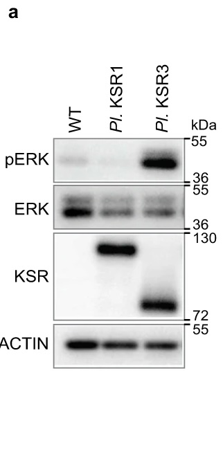
The authors of this publication knew that in sea urchin development, activation of the ERK pathway is important, but also occurs through a mechanism that is different from the few ways scientists normally see ERK activated. Through an RNA-seq screen, they identified the gene ksr3 as a candidate for the ERK activator. One experiment they performed to verify this result is shown. They overexpressed sea urchin KSR3 or the related protein KSR1 in human epithelial cells in culture, then made cell lysates for use in the western blot. The researchers wanted to measure ERK phosphorylation, since phosphorylated ERK is the active form. The labels on the top show which sample was run in each lane, whereas the samples on the side show which antibody was used in that piece of the blot. Note that the pERK and ERK antibodies recognize the closely related and similarly sized proteins ERK1 and ERK2, which is why those blots have two closely spaced bands. The top blot shows that there is far more phospho-ERK, i.e. active ERK, in the KSR3-containing sample than the control or the KSR1 sample. The second blot shows that there is actually a decrease in total ERK when KSR1 and 3 are present compared to the control. The third blot uses an antibody that recognizes both KSR1 and KSR3, which are different sizes. This blot just shows that the overexpression was successful. Lastly, actin is a loading control, showing that approximately the same amount of lysate was loaded in each lane. Since there is far more pERK and less ERK in the KSR3 sample compared to the other samples, KSR3 is responsible for activating ERK.
Image Descriptions
Figure 1 image description:
A western blot.
|
WT |
Pl. KSR1 |
Pl. KSR3 |
|
|---|---|---|---|
|
pERK |
Almost no signal |
Almost no signal |
Strong signal |
|
ERK |
Strong signal, 2 bands |
~50% of wt signal, 2 bands |
~50% of wt signal, 2 bands |
|
KSR |
No signal |
Signal further up membrane (larger protein size), similar intensity to KSR3 |
Signal further down membrane (smaller protein size), similar intensity to KSR1 |
|
Actin |
Approximately equal signal across all lanes |
||
Thumbnails
"Rice Genetics III_p789a"↗ by IRRI Photos is licensed under CC BY-NC-SA 2.0↗.
Description: Western blot.
Author
Katherine Mattaini, Tufts University
-
Chessel, A., N. De Crozé, M. D. Molina, L. Taberner, P. Dru, L. Martin, and T. Lepage. 2023. RAS-independent ERK activation by constitutively active KSR3 in non-chordate metazoa. Nature Communications 14:3970. ↵