
29: Sanger Sequencing
- Page ID
- 172081
\( \newcommand{\vecs}[1]{\overset { \scriptstyle \rightharpoonup} {\mathbf{#1}} } \)
\( \newcommand{\vecd}[1]{\overset{-\!-\!\rightharpoonup}{\vphantom{a}\smash {#1}}} \)
\( \newcommand{\dsum}{\displaystyle\sum\limits} \)
\( \newcommand{\dint}{\displaystyle\int\limits} \)
\( \newcommand{\dlim}{\displaystyle\lim\limits} \)
\( \newcommand{\id}{\mathrm{id}}\) \( \newcommand{\Span}{\mathrm{span}}\)
( \newcommand{\kernel}{\mathrm{null}\,}\) \( \newcommand{\range}{\mathrm{range}\,}\)
\( \newcommand{\RealPart}{\mathrm{Re}}\) \( \newcommand{\ImaginaryPart}{\mathrm{Im}}\)
\( \newcommand{\Argument}{\mathrm{Arg}}\) \( \newcommand{\norm}[1]{\| #1 \|}\)
\( \newcommand{\inner}[2]{\langle #1, #2 \rangle}\)
\( \newcommand{\Span}{\mathrm{span}}\)
\( \newcommand{\id}{\mathrm{id}}\)
\( \newcommand{\Span}{\mathrm{span}}\)
\( \newcommand{\kernel}{\mathrm{null}\,}\)
\( \newcommand{\range}{\mathrm{range}\,}\)
\( \newcommand{\RealPart}{\mathrm{Re}}\)
\( \newcommand{\ImaginaryPart}{\mathrm{Im}}\)
\( \newcommand{\Argument}{\mathrm{Arg}}\)
\( \newcommand{\norm}[1]{\| #1 \|}\)
\( \newcommand{\inner}[2]{\langle #1, #2 \rangle}\)
\( \newcommand{\Span}{\mathrm{span}}\) \( \newcommand{\AA}{\unicode[.8,0]{x212B}}\)
\( \newcommand{\vectorA}[1]{\vec{#1}} % arrow\)
\( \newcommand{\vectorAt}[1]{\vec{\text{#1}}} % arrow\)
\( \newcommand{\vectorB}[1]{\overset { \scriptstyle \rightharpoonup} {\mathbf{#1}} } \)
\( \newcommand{\vectorC}[1]{\textbf{#1}} \)
\( \newcommand{\vectorD}[1]{\overrightarrow{#1}} \)
\( \newcommand{\vectorDt}[1]{\overrightarrow{\text{#1}}} \)
\( \newcommand{\vectE}[1]{\overset{-\!-\!\rightharpoonup}{\vphantom{a}\smash{\mathbf {#1}}}} \)
\( \newcommand{\vecs}[1]{\overset { \scriptstyle \rightharpoonup} {\mathbf{#1}} } \)
\(\newcommand{\longvect}{\overrightarrow}\)
\( \newcommand{\vecd}[1]{\overset{-\!-\!\rightharpoonup}{\vphantom{a}\smash {#1}}} \)
\(\newcommand{\avec}{\mathbf a}\) \(\newcommand{\bvec}{\mathbf b}\) \(\newcommand{\cvec}{\mathbf c}\) \(\newcommand{\dvec}{\mathbf d}\) \(\newcommand{\dtil}{\widetilde{\mathbf d}}\) \(\newcommand{\evec}{\mathbf e}\) \(\newcommand{\fvec}{\mathbf f}\) \(\newcommand{\nvec}{\mathbf n}\) \(\newcommand{\pvec}{\mathbf p}\) \(\newcommand{\qvec}{\mathbf q}\) \(\newcommand{\svec}{\mathbf s}\) \(\newcommand{\tvec}{\mathbf t}\) \(\newcommand{\uvec}{\mathbf u}\) \(\newcommand{\vvec}{\mathbf v}\) \(\newcommand{\wvec}{\mathbf w}\) \(\newcommand{\xvec}{\mathbf x}\) \(\newcommand{\yvec}{\mathbf y}\) \(\newcommand{\zvec}{\mathbf z}\) \(\newcommand{\rvec}{\mathbf r}\) \(\newcommand{\mvec}{\mathbf m}\) \(\newcommand{\zerovec}{\mathbf 0}\) \(\newcommand{\onevec}{\mathbf 1}\) \(\newcommand{\real}{\mathbb R}\) \(\newcommand{\twovec}[2]{\left[\begin{array}{r}#1 \\ #2 \end{array}\right]}\) \(\newcommand{\ctwovec}[2]{\left[\begin{array}{c}#1 \\ #2 \end{array}\right]}\) \(\newcommand{\threevec}[3]{\left[\begin{array}{r}#1 \\ #2 \\ #3 \end{array}\right]}\) \(\newcommand{\cthreevec}[3]{\left[\begin{array}{c}#1 \\ #2 \\ #3 \end{array}\right]}\) \(\newcommand{\fourvec}[4]{\left[\begin{array}{r}#1 \\ #2 \\ #3 \\ #4 \end{array}\right]}\) \(\newcommand{\cfourvec}[4]{\left[\begin{array}{c}#1 \\ #2 \\ #3 \\ #4 \end{array}\right]}\) \(\newcommand{\fivevec}[5]{\left[\begin{array}{r}#1 \\ #2 \\ #3 \\ #4 \\ #5 \\ \end{array}\right]}\) \(\newcommand{\cfivevec}[5]{\left[\begin{array}{c}#1 \\ #2 \\ #3 \\ #4 \\ #5 \\ \end{array}\right]}\) \(\newcommand{\mattwo}[4]{\left[\begin{array}{rr}#1 \amp #2 \\ #3 \amp #4 \\ \end{array}\right]}\) \(\newcommand{\laspan}[1]{\text{Span}\{#1\}}\) \(\newcommand{\bcal}{\cal B}\) \(\newcommand{\ccal}{\cal C}\) \(\newcommand{\scal}{\cal S}\) \(\newcommand{\wcal}{\cal W}\) \(\newcommand{\ecal}{\cal E}\) \(\newcommand{\coords}[2]{\left\{#1\right\}_{#2}}\) \(\newcommand{\gray}[1]{\color{gray}{#1}}\) \(\newcommand{\lgray}[1]{\color{lightgray}{#1}}\) \(\newcommand{\rank}{\operatorname{rank}}\) \(\newcommand{\row}{\text{Row}}\) \(\newcommand{\col}{\text{Col}}\) \(\renewcommand{\row}{\text{Row}}\) \(\newcommand{\nul}{\text{Nul}}\) \(\newcommand{\var}{\text{Var}}\) \(\newcommand{\corr}{\text{corr}}\) \(\newcommand{\len}[1]{\left|#1\right|}\) \(\newcommand{\bbar}{\overline{\bvec}}\) \(\newcommand{\bhat}{\widehat{\bvec}}\) \(\newcommand{\bperp}{\bvec^\perp}\) \(\newcommand{\xhat}{\widehat{\xvec}}\) \(\newcommand{\vhat}{\widehat{\vvec}}\) \(\newcommand{\uhat}{\widehat{\uvec}}\) \(\newcommand{\what}{\widehat{\wvec}}\) \(\newcommand{\Sighat}{\widehat{\Sigma}}\) \(\newcommand{\lt}{<}\) \(\newcommand{\gt}{>}\) \(\newcommand{\amp}{&}\) \(\definecolor{fillinmathshade}{gray}{0.9}\)Sanger sequencing is a sequencing-by-synthesis method used to determine the nucleotide sequence of a short molecule of DNA. Sanger sequencing is appropriate when the length of the DNA molecule to be sequenced is 100-1000 nt.
Also known as:
Dideoxy sequencing
Chain termination method
Samples needed
To perform Sanger sequencing, you need:
- DNA template
- DNA oligonucleotide primer that anneals to the 3’ end of the DNA template. In the manual version of Sanger sequencing, the primer is radioactively labeled.
- Solution of dNTPs
- Solutions of each of the 4 dideoxynucleotide triphosphates (ddNTPs). In automated Sanger sequencing, each of the 4 types of ddNTPs is labeled with a different colored fluorophore.
- DNA polymerase
- Polyacrylamide gel electrophoresis apparatus (for manual sequencing) or a machine that reads Sanger sequencing reaction products using capillary gel electrophoresis and a laser detector (for automated sequencing)
Method
Sanger sequencing is a specialized DNA synthesis reaction invented by Fred Sanger. The original method used radioactively labeled DNA molecules and polyacrylamide gel electrophoresis. In modern, automated Sanger sequencing, a double-stranded DNA molecule to be sequenced is incubated with a primer that anneals to its 3’ terminus, dNTPs, fluorescently labeled ddNTPs (each type of ddNTP is labeled with a different fluorophore), and a DNA polymerase (Fig. 1). The concentration of the ddNTPs is much lower than the concentration of the dNTPs, so there is a small probability that a ddNTP will be incorporated opposite its complementary base at each position. Once the reaction is completed, the products consist of a collection of fragments, each labeled at its 3’ end with a fluorophore corresponding to the ddNTP that terminated the synthesis reaction. These fragments are separated using capillary gel electrophoresis and the fluorophore present on each molecule is detected. A computer processes the data to create a chromatogram that shows the DNA sequence that was synthesized. The sequence of the original DNA template is the reverse complement.
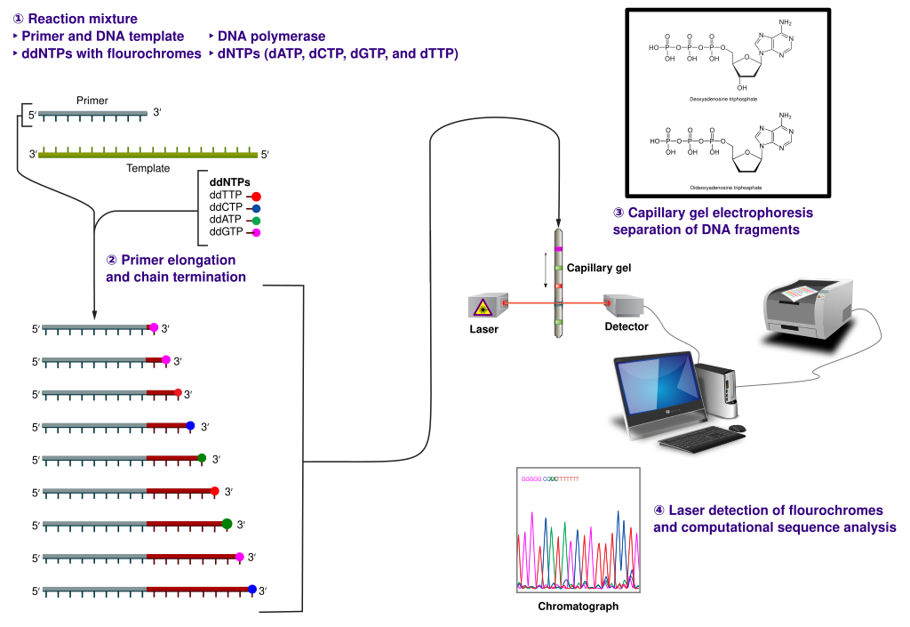 Figure 1. Sanger sequencing using fluorescently labeled ddNTPs. For details, see “Method.” "Sanger-sequencing"↗ by Estevezj↗ is licensed under CC BY-SA 3.0↗. [Image description]
Controls
Typically, no controls are used for Sanger sequencing. Sometimes, the DNA template is sequenced from both directions (using primers that anneal to each end of the double-strand template), and the sequence output is compared for consistency.
Interpretation

This figure shows the results of Sanger DNA sequencing reactions using a dystrophin gene fragment as a template, a radioactively labeled primer, and ddATP, ddGTP, ddTTP, and ddCTP in four separate reactions, for two individuals side-by-side. The individual without muscular dystrophy has a G at position 35, while the individual with muscular dystrophy has a T at this position. The sequence is read from the bottom of the gel to the top of the gel, with the smaller fragments corresponding to synthesis reactions that terminated early near the 3’ end of the template.

This figure shows the chromatograms for four family members, including an individual with muscular dystrophy. The patient has a peak corresponding to a synthesis fragment that terminated with a T, while their brother and father have peaks corresponding to C (which is the same as the control sequence). The mother is heterozygous for the T and C peaks. The patient inherited the chromosome with the T peak from his mother.
Image descriptions
Figure 1 image description:
A diagram of automated Sanger sequencing using fluorescently labeled ddNTPs. ↵
Figure 2 image description:
The results of a sequencing gel used to separate DNA synthesis products of the dystrophin gene, created using radioactively labeled primers in separate Sanger sequencing reactions with four different ddNTPs. There is a single difference in the sequences between the two individuals, with the muscular dystrophy patient having a T where the arrow is pointing. ↵
Figure 3 image description:
The results of five automated Sanger sequencing reactions giving portions of the dystrophin gene sequence for a control sample and four family members. The base calls are represented by peaks at each position within the gene. The sequence corresponding to the peaks is written below each line, with the corresponding positions indicated by numbers. The differences in the sequences are indicated by arrows. ↵
Thumbnail
"Skraban–Deardorff syndrome — Sanger sequencing (cropped)"↗ by Jiacheng Hu; Mingming Xu; Xiaobo Zhu; Yu Zhang is licensed under CC BY 4.0↗.
Author
Mitch McVey, Tufts University
1. Chaturvedi, L. S., M. Mukherjee, S. Srivastava, E. D. Mittal, and B. Mittal. 2001. Point mutation and polymorphism in Duchenne/Becker Muscular Dystrophy (D/BMD) patients. Experimental and Molecular Medicine 33: 251-256. Return to Figure 2. Return to Figure 3.