
26: Quantitative Real Time PCR
- Page ID
- 141656
\( \newcommand{\vecs}[1]{\overset { \scriptstyle \rightharpoonup} {\mathbf{#1}} } \)
\( \newcommand{\vecd}[1]{\overset{-\!-\!\rightharpoonup}{\vphantom{a}\smash {#1}}} \)
\( \newcommand{\dsum}{\displaystyle\sum\limits} \)
\( \newcommand{\dint}{\displaystyle\int\limits} \)
\( \newcommand{\dlim}{\displaystyle\lim\limits} \)
\( \newcommand{\id}{\mathrm{id}}\) \( \newcommand{\Span}{\mathrm{span}}\)
( \newcommand{\kernel}{\mathrm{null}\,}\) \( \newcommand{\range}{\mathrm{range}\,}\)
\( \newcommand{\RealPart}{\mathrm{Re}}\) \( \newcommand{\ImaginaryPart}{\mathrm{Im}}\)
\( \newcommand{\Argument}{\mathrm{Arg}}\) \( \newcommand{\norm}[1]{\| #1 \|}\)
\( \newcommand{\inner}[2]{\langle #1, #2 \rangle}\)
\( \newcommand{\Span}{\mathrm{span}}\)
\( \newcommand{\id}{\mathrm{id}}\)
\( \newcommand{\Span}{\mathrm{span}}\)
\( \newcommand{\kernel}{\mathrm{null}\,}\)
\( \newcommand{\range}{\mathrm{range}\,}\)
\( \newcommand{\RealPart}{\mathrm{Re}}\)
\( \newcommand{\ImaginaryPart}{\mathrm{Im}}\)
\( \newcommand{\Argument}{\mathrm{Arg}}\)
\( \newcommand{\norm}[1]{\| #1 \|}\)
\( \newcommand{\inner}[2]{\langle #1, #2 \rangle}\)
\( \newcommand{\Span}{\mathrm{span}}\) \( \newcommand{\AA}{\unicode[.8,0]{x212B}}\)
\( \newcommand{\vectorA}[1]{\vec{#1}} % arrow\)
\( \newcommand{\vectorAt}[1]{\vec{\text{#1}}} % arrow\)
\( \newcommand{\vectorB}[1]{\overset { \scriptstyle \rightharpoonup} {\mathbf{#1}} } \)
\( \newcommand{\vectorC}[1]{\textbf{#1}} \)
\( \newcommand{\vectorD}[1]{\overrightarrow{#1}} \)
\( \newcommand{\vectorDt}[1]{\overrightarrow{\text{#1}}} \)
\( \newcommand{\vectE}[1]{\overset{-\!-\!\rightharpoonup}{\vphantom{a}\smash{\mathbf {#1}}}} \)
\( \newcommand{\vecs}[1]{\overset { \scriptstyle \rightharpoonup} {\mathbf{#1}} } \)
\(\newcommand{\longvect}{\overrightarrow}\)
\( \newcommand{\vecd}[1]{\overset{-\!-\!\rightharpoonup}{\vphantom{a}\smash {#1}}} \)
\(\newcommand{\avec}{\mathbf a}\) \(\newcommand{\bvec}{\mathbf b}\) \(\newcommand{\cvec}{\mathbf c}\) \(\newcommand{\dvec}{\mathbf d}\) \(\newcommand{\dtil}{\widetilde{\mathbf d}}\) \(\newcommand{\evec}{\mathbf e}\) \(\newcommand{\fvec}{\mathbf f}\) \(\newcommand{\nvec}{\mathbf n}\) \(\newcommand{\pvec}{\mathbf p}\) \(\newcommand{\qvec}{\mathbf q}\) \(\newcommand{\svec}{\mathbf s}\) \(\newcommand{\tvec}{\mathbf t}\) \(\newcommand{\uvec}{\mathbf u}\) \(\newcommand{\vvec}{\mathbf v}\) \(\newcommand{\wvec}{\mathbf w}\) \(\newcommand{\xvec}{\mathbf x}\) \(\newcommand{\yvec}{\mathbf y}\) \(\newcommand{\zvec}{\mathbf z}\) \(\newcommand{\rvec}{\mathbf r}\) \(\newcommand{\mvec}{\mathbf m}\) \(\newcommand{\zerovec}{\mathbf 0}\) \(\newcommand{\onevec}{\mathbf 1}\) \(\newcommand{\real}{\mathbb R}\) \(\newcommand{\twovec}[2]{\left[\begin{array}{r}#1 \\ #2 \end{array}\right]}\) \(\newcommand{\ctwovec}[2]{\left[\begin{array}{c}#1 \\ #2 \end{array}\right]}\) \(\newcommand{\threevec}[3]{\left[\begin{array}{r}#1 \\ #2 \\ #3 \end{array}\right]}\) \(\newcommand{\cthreevec}[3]{\left[\begin{array}{c}#1 \\ #2 \\ #3 \end{array}\right]}\) \(\newcommand{\fourvec}[4]{\left[\begin{array}{r}#1 \\ #2 \\ #3 \\ #4 \end{array}\right]}\) \(\newcommand{\cfourvec}[4]{\left[\begin{array}{c}#1 \\ #2 \\ #3 \\ #4 \end{array}\right]}\) \(\newcommand{\fivevec}[5]{\left[\begin{array}{r}#1 \\ #2 \\ #3 \\ #4 \\ #5 \\ \end{array}\right]}\) \(\newcommand{\cfivevec}[5]{\left[\begin{array}{c}#1 \\ #2 \\ #3 \\ #4 \\ #5 \\ \end{array}\right]}\) \(\newcommand{\mattwo}[4]{\left[\begin{array}{rr}#1 \amp #2 \\ #3 \amp #4 \\ \end{array}\right]}\) \(\newcommand{\laspan}[1]{\text{Span}\{#1\}}\) \(\newcommand{\bcal}{\cal B}\) \(\newcommand{\ccal}{\cal C}\) \(\newcommand{\scal}{\cal S}\) \(\newcommand{\wcal}{\cal W}\) \(\newcommand{\ecal}{\cal E}\) \(\newcommand{\coords}[2]{\left\{#1\right\}_{#2}}\) \(\newcommand{\gray}[1]{\color{gray}{#1}}\) \(\newcommand{\lgray}[1]{\color{lightgray}{#1}}\) \(\newcommand{\rank}{\operatorname{rank}}\) \(\newcommand{\row}{\text{Row}}\) \(\newcommand{\col}{\text{Col}}\) \(\renewcommand{\row}{\text{Row}}\) \(\newcommand{\nul}{\text{Nul}}\) \(\newcommand{\var}{\text{Var}}\) \(\newcommand{\corr}{\text{corr}}\) \(\newcommand{\len}[1]{\left|#1\right|}\) \(\newcommand{\bbar}{\overline{\bvec}}\) \(\newcommand{\bhat}{\widehat{\bvec}}\) \(\newcommand{\bperp}{\bvec^\perp}\) \(\newcommand{\xhat}{\widehat{\xvec}}\) \(\newcommand{\vhat}{\widehat{\vvec}}\) \(\newcommand{\uhat}{\widehat{\uvec}}\) \(\newcommand{\what}{\widehat{\wvec}}\) \(\newcommand{\Sighat}{\widehat{\Sigma}}\) \(\newcommand{\lt}{<}\) \(\newcommand{\gt}{>}\) \(\newcommand{\amp}{&}\) \(\definecolor{fillinmathshade}{gray}{0.9}\)Summary
Quantitative real time PCR (qRT-PCR) is used to determine the amount of a specific DNA sequence in a DNA mixture.
Also known as
qRT-PCR, qPCR, real time PCR
Note that the acronym RT-PCR can be confusing, as both real time and reverse transcription PCR can be abbreviated “RT,” so care should be taken to avoid confusion.
Samples needed
Sample of DNA, with a mixture of sequences
Method
qRT-PCR is a quantitative variant of typical PCR. It is used to determine how much of a particular DNA sequence is present in a mixture. This can be used to determine gene expression levels (following RT-PCR of cellular RNAs), gene copy number, and for other applications.
With a pair of primers that amplify the target DNA, the amount of the target should double in each PCR cycle. The principle of qRT-PCR is that the less abundant the target DNA sequence in the sample, the more cycles it will take for the abundance of the target to reach a certain threshold. The number of cycles required to reach the threshold is known as the Ct value. Therefore, in two samples, the one with a lower Ct value indicates that the target DNA is more abundant in that sample.
In order to track the production of target DNA in real time, qRT-PCR uses a special machine that can detect fluorescence over the course of the PCR program. In addition to the usual PCR reagents, qRT-PCR requires a method for tracking production of the target. One method uses dyes that only fluoresce when they bind to dsDNA. This is the case for the popular reagent SYBR green. The second method uses probes that are specific to the target DNA sequence and which only fluoresce when they are cleaved by Taq DNA polymerase. These are called Taqman probes. Each of these methods has benefits and drawbacks. In both cases, a certain fluorescence signal is chosen as the threshold value.
qRT-PCR data is either compared to a standard curve or to an internal reference sample to determine absolute or relative DNA quantities, respectively.
Controls
As with any PCR protocol, primer specificity should be considered. If using intercalating dyes like SYBR green, a melt curve can be used to determine how many PCR products are produced in each reaction. After the normal PCR program runs, the temperature of the mixture is raised, and the change in fluorescence is monitored. When a product’s melting temperature is reached, there is a peak in the ΔF signal. More than one peak in the melt curve indicates that the primers are not entirely specific.
When using qRT-PCR to measure gene expression, an endogenous control sequence is often amplified in addition to the sequence of interest. The endogenous control should be a gene whose expression is known to be very stable and is not affected by experimental treatments. This can be used to normalize the signal from the sequence of interest (to account for small differences in total cDNA added). Other controls relating to the reverse transcription step should also be used.
Furthermore, sometimes a no template control (water instead of DNA sample) is used to ensure that none of the other reagents are contaminated with DNA.
Interpretation
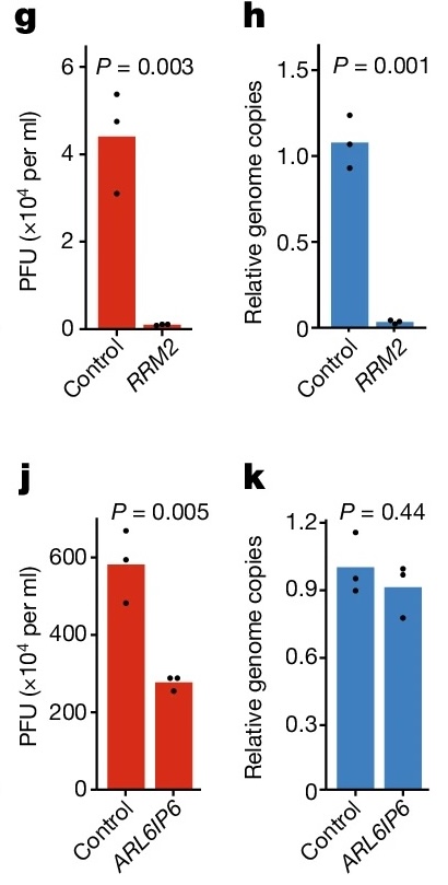 Figure 1. Virus production (left, red) and genomic copy number (right, blue) of human cytomegalovirus (HCMV) in the context of CRISPR-generated host gene knockouts. Relevant section of caption for published figure reads: “g,j, RRM2-knockout (g), ARL6IP6-knockout (j) and control cells were infected with HCMV-GFP virus. At 7 dpi viral supernatant was used to infect recipient wild-type fibroblasts. Forty-eight hours later, the percentage of GFP-positive recipient cells was determined by flow cytometry and used to calculate the number of plaque-forming units (PFU). n = 3 biological replicates. h,k. DNA was extracted from RRM2-knockout (h), ARL6IP6-knockout (k) and control cells infected with HCMV at 3 dpi and viral DNA was quantified using quantitative PCR (qPCR) and normalized to host DNA. n = 3 biological replicates. ” “Figure 2” by Finkel et al.[1]. [Image description]
In this experiment, researchers performed a CRISPR-generated knockout screen to ask what host cell genes are involved in human cytomegalovius (HCMV) infection. Two knockouts are shown: RRM2 in the top row & ARL6IP6 in the bottom row. In panels g & j (left, red), the plaque-forming units (PFU) generated in each type of knockout cell are shown. PFU correlates with the number of viral particles that can infect new cells. Both knockouts significantly reduce the amount of functional viral particles formed. Panels h & k (right, blue) show the results of a qRT-PCR experiment to quantify the relative number of HCMV genome copies in each knockout cell compared to controls. While RRM2 knockout almost completely abrogates the ability of HCMV to copy its genome, ARL6IP6 does not significantly affect HCMV viral copy number. Therefore, ARL6IP6 mainly acts on a step other than viral genome copying.
Image Descriptions
Figure 1 image description:
Four column graphs. Panels g and j measure PFU in various samples. Panel g shows ~4.3 x 10⁴ PFU per ml in control cells and almost 0 in RRM2 knockout cells with p = 0.003. Panel j shows ~580 x 104 PFU per ml in control cells and ~270 x 104 PFU per ml in ARL6IP6 knockout cells with p - 0.005. Panels h and k show relative genome copies compared to control cells. Panel h shows nearly 0 genome copies in RRM2 knockout cells with p = 0.001, and panel k shows ~0. 85 genome copies in ARL6IP6 knockout cells with p = 0.044. ↵
Thumbnail
"Qpcr-cycling.png"↗ by Zuzanna K. Filutowska is licensed under CC BY-SA 3.0↗.
Description: qPCR amplification plot.
Author
Katherine Mattaini, Tufts University
-
Finkel, Y., A. Nachshon, E. Aharon, T. Arazi, E. Simonovsky, M. Dobešová, Z. Saud, A. Gluck, T. Fisher, R. J. Stanton, M. Schwartz, and N. Stern-Ginossar. 2024. A virally encoded high-resolution screen of cytomegalovirus dependencies. Nature 630:712–719. ↵