Helena-Test

Exercise \(\PageIndex{1}\)

Degradation of amino acids yields compounds that are common intermediates in the major   metabolic pathways. Explain the distinction between glucogenic and ketogenic amino acids in terms of their metabolic fates.

Answer

Glucogenic amino acids are those which can be catabolized into pyruvate, oxaloacetate, a-ketoglutarate , fumarate, or succinyl-CoA, and thus can serve as glucose precursors.

Ketogenic amino acids are catabolized to Acetyl-CoA or acetoacetate, and thus can serve as precursors for fatty acids or ketone bodies.

 

Here is a hint if you need it.

 

Authored by Helena Prieto.  Last update:  06.05.23

Date of origin 06.05.23

Introduction

[ADD CONTENT]

New Heading  

[ADD TEXT]

 

 

[ADD IMAGE] (saved to your computer and uploaded with picture icon from top menu bar or drag image file to location (required from svg image)

*Use the following under your picture:

Figure \(\PageIndex{x}\): [Add caption]

*Center Picture and Caption together using top menu bar

 

[ADD iCn3D Model]

 

 

 

[ADD MATHEMATIC GRAPH - REUSE]

*your text and graph

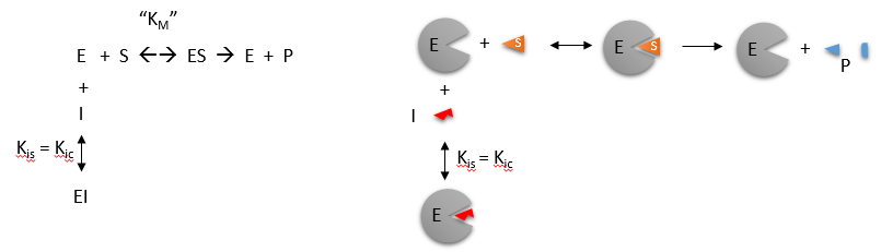
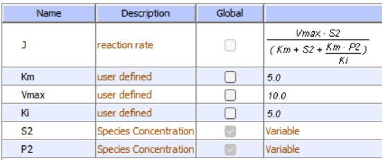
Reversible Competitive inhibition occurs when substrate (S) and inhibitor (I) both bind to the same site on the enzyme. In effect, they compete for the active site and bind in a mutually exclusive fashion. This is illustrated in the chemical equations and molecular cartoons shown in Figure \(\PageIndex{1}\).

Figure \(\PageIndex{1}\): Competitive Inhibition

\begin{equation}
v_0=\frac{V_M S}{K_M\left(1+\frac{I}{K is}\right)+S}
\end{equation}

There is another type of inhibition that would give the same kinetic data. If S and I bound to different sites, and S bound to E and produced a conformational change in E such that I could not bind (and vice versa), then the binding of S and I would be mutually exclusive. This is called allosteric competitive inhibition. Inhibition studies are usually done at several fixed and non-saturating concentrations of I and varying S concentrations.

The key kinetic parameters to understand are V_M and K_M. Let us assume for ease of equation derivation that I binds reversibly, and with rapid equilibrium to E, with a dissociation constant K_IS. The "s" in the subscript "is" indicates that the slope of the 1/v vs 1/S Lineweaver-Burk plot changes while the y-intercept stays constant. K_IS is also named K_IC where the subscript "c" stands for competitive inhibition constant.

A look at the top mechanism shows that even in the presence of I, as S increases to infinity, all E is converted to ES. That is, there is no free E to which I could bind. Now, remember that V_M= k_catE₀. Under these conditions, ES = E₀; hence v = V_M. V_M is not changed. However, the apparent K_M, K_Mapp, will change. We can use LaChatelier's principle to understand this. If I binds to E alone and not ES, it will shift the equilibrium of E + S → ES to the left. This would increase the K_Mapp (i.e. it would appear that the affinity of E and S has decreased.). The double reciprocal plot (Lineweaver-Burk plot) offers a great way to visualize the inhibition as shown in Figure \(\PageIndex{2}\).

Figure \(\PageIndex{2}\): Competitive Inhibition: Lineweaver-Burk plots

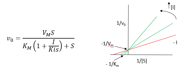
In the presence of I, V_M does not change, but K_M appears to increase. Therefore, 1/K_M, the x-intercept on the plot will get smaller, and closer to 0. Therefore the plots will consist of a series of lines, with the same y-intercept (1/V_M), and the x-intercepts (-1/K_M) closer and closer to 0 as I increases. These intersecting plots are the hallmark of competitive inhibition.

Here is an interactive graph showing v₀ vs [S] for competitive inhibition with Vm and Km both set to 100. Change the sliders for [I] and Kis and see the effect on the graph.

Here is the interactive graphs showing 1/v₀ vs 1/[S] for competitive inhibition, with Vm and Km both set to 10.

Note that in the first three inhibition models discussed in this section, the Lineweaver-Burk plots are linear in the presence and absence of an inhibitor. This suggests that plots of v vs S in each case would be hyperbolic and conform to the usual form of the Michaelis Menton equation, each with potentially different apparent V_M and K_M values.

An equation for v₀ in the presence of a competitive inhibitor is shown in the above figure. The only change compared to the equation for the initial velocity in the absence of the inhibitor is that the K_M term is multiplied by the factor 1+I/K_is. Hence K_Mapp = K_M(1+I/Kis). This shows that the apparent K_M does increase as we predicted. K_IS is the inhibitor dissociation constant in which the inhibitor affects the slope of the double reciprocal plot.

v₀ vs log [Inhibitor] plots

If the data were plotted as v₀ vs log S, the plots would be sigmoidal, as we saw for plots of ML vs log L in Chapter 5B. In the case of a competitive inhibitor, the plot of v₀ vs log S in the presence of different fixed concentrations of inhibitor would consist of a series of sigmoidal curves, each with the same V_M, but with different apparent K_M values (where K_Mapp = K_M(1+I/K_is), progressively shifted to the right. Enzyme kinetic data is rarely plotted this way. These plots are mostly used for simple binding data for the M + L ↔ ML equilibrium, in the presence of different inhibitor concentrations.

Reconsider our discussion of the simple binding equilibrium, M + L ↔ ML. For fractional saturation Y vs a log L graphs, we considered three examples:

1. L = 0.01 K_D (i.e. L << K_D), which implies that K_D = 100L. Then Y = L/[K_D+L] = L/[100L + L] ≈1/100. This implies that irrespective of the actual [L], if L = 0.01 K_D, then Y ≈0.01.
2. L = 100 K_D (i.e. L >> K_D), which implies that K_D = L/100. Then Y = L/[K_D+L] = L/[(L/100) + L] = 100L/101L ≈ 1. This implies that irrespective of the actual [L], if L = 100 Kd, then Y ≈1.
3. L = K_D, then Y = 0.5

These scenarios show that if L varies over 4 orders of magnitude (0.01K_D < K_D < 100K_D), or, in log terms, from
-2 + log K_D < log K_D< 2 + log Kd), irrespective of the magnitude of the K_D, that Y varies from approximately 0 - 1.

In other words, Y varies from 0-1 when L varies from log K_D by +2. Hence, plots of Y vs log L for a series of binding reactions of increasingly higher K_D (lower affinity) would reveal a series of identical sigmoidal curves shifted progressively to the right, as shown below in Figure \(\PageIndex{3}\).

Figure \(\PageIndex{3}\): Plot of fractional saturation Y vs log L for two different K_D values.

The same would be true of v₀ vs S in the presence of different concentrations of a competitive inhibitor, for initial flux, Jo vs ligand outside, in the presence of a competitive inhibitor, or ML vs L (or Y vs L) in the presence of a competitive inhibitor.

In many ways plots of v₀ vs lnS are easier to visually interpret than plots of v₀ vs S . As noted for simple binding plots, textbook illustrations of hyperbolas are often misdrawn, showing curves that level off too quickly as a function of [S] as compared to plots of v₀ vs lnS, in which it is easy to see if saturation has been achieved. In addition, as the curves above show, multiple complete plots of v₀ vs lnS at varying fixed inhibitor concentrations or for variant enzyme forms (different isoforms, site-specific mutants) over a broad range of lnS can be made which facilitates comparisons of the experimental kinetics under these different conditions. This is especially true if Km values differ widely.

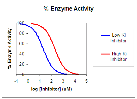
Now that you are more familiar with binding and enzyme kinetics curves, in the presence and absence of inhibitors, you should be able to apply the above analysis to inhibition curves where the binding or the initial velocity is plotted at varying competitive inhibitor concentrations at different fixed nonsaturating concentrations of ligand or substrate. Consider the activity of an enzyme. Let's say that at some reasonable concentration of substrate (not infinite), the enzyme is approximately 100% active. If a competitive inhibitor is added, the activity of the enzyme decreases until at saturating (infinite) I, no activity would remain. Graphs showing this are shown below in Figure \(\PageIndex{4}\).

Figure \(\PageIndex{4}\): Inhibition of Enzyme Activity - % Activity vs log [Inhibitor]

Progress Curves for Competitive Inhibition

In the previous section, we explored how important progress curve (Product vs time) analyses are in understanding both uncatalyzed and enzyme-catalyzed reactions. We are aware of no textbooks which cover progress curves for enzyme inhibition. Yet progress curves are what most investigators record and analyze to determine initial rates v₀ and to calculate V_M, K_M and inhibition constants, as described above. We will use Vcell to produce progress curves for reversibly inhibited enzyme-catalyzed reactions.

---

MODEL

Competitive Inhibition with constant [I]:   

No inhibition (left) and competitive inhibition (right)

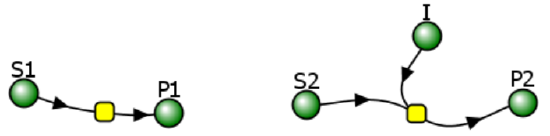
Initial conditions for no inhibition

Initial conditions for competitive inhibition

I is fixed for each simulation (as it is not converted to a product) but can be changed in the simulation below.

Select Load [model name] below

 Select Start to begin the simulation.

Interactive Element

Select Plot to change Y axis min/max, then Reset and Play  |  Select Slider to change which constants are displayed.  For this model, select Vm, Km, Ki and I |  Select About  for software information.

Move the sliders to change the constants and see changes in the displayed graph in real-time. 

Time course model made using Virtual Cell (Vcell), The Center for Cell Analysis & Modeling, at UConn Health.  Funded by NIH/NIGMS (R24 GM137787); Web simulation software (miniSidewinder) from Bartholomew Jardine and Herbert M. Sauro, University of Washington.  Funded by NIH/NIGMS (RO1-GM123032-04)

---

 

The graphs from your initial run show the concentrations of S, P and I as a function of time for just the initial conditions shown above. In typical initial rate laboratory analyzes, of competitive inhibition, at least three sets of reactions are run with the same varying substrate concentrations and different fixed concentrations of inhibitor. In the analyses above, [I] is fixed at 5 uM.

Conduct a series of run at different values of I. Vary the K_I, the dissociation constant for the EI complex, as follows:

• I << K_I, the dissociation constant for the EI complex
• I >> K_I, the dissociation constant for the EI complex. Then download the data and determine the initial rate for each of the initial conditions.

 

Figure \(\PageIndex{5}\) shows an interactive iCn3D model of human low molecular weight phosphotyrosyl phosphatase bound to a competitive inhibitor (5PNT)

Figure \(\PageIndex{5}\): Human low molecular weight phosphotyrosyl phosphatase bound to a competitive inhibitor (5PNT). (Copyright; author via source).
Click the image for a popup or use this external link: https://structure.ncbi.nlm.nih.gov/i...XsEacG2tixDDi9

The competitive inhibitor, the deprotonated form of 2-(N-morpholino)-ethanesulfonic acid (MES), is actually the conjugate base of the weak acid (pKa = 6.15) of a commonly used component of a buffered solution.  It is shown in color sticks with the negatively charged sulfonate sitting at the bottom of the active site pocket.  The amino acids comprising the active site binding pocket are shown as color sticks underneath the transparent colored surface of the binding pocket.  The normal substrates for the enzyme are proteins phosphorylated on tyrosine side chains so the sulfonate is a mimic of the negatively charged phosphate group of the phosphoprotein target.

 

Two specials cases of competition inhibition

Product Inhibition

Let's look at an enzyme that converts reactant S to product P. Since P arises from S, they may have structural similarities. For example, what if GTP was the reactant and GDP was a product? If so, then P might also bind in the active site and inhibit the conversion of S to P. This is called product inhibition. It probably occurs in most enzymes, and when it does occur it will start bending downward the beginning part of the progress curve for P formation. If the product binds very tightly, it might cause a significant underestimation of the initial velocity (v₀) or flux (J₀) of the enzyme. Let's use Vcell to explore product inhibition. The model will explore two reactions:

• E + R ↔ ER → E + Q (no product inhibition)
• E + S ↔ ES → E + P (with product inhibition)

Note that the chemical equation above does not explicitly show the product P binding the enzyme to form an EP complex. An actual reaction diagram showing the inhibition of an enzyme by an inhibitor I and by the product P is shown in Figure \(\PageIndex{6}\) below.

Figure \(\PageIndex{6}\): reaction diagram showing inhibition of an enzyme by an inhibitor I and by the product P

Vcell uses much simpler diagrams since it is most often used for modeling whole pathways or even entire cells. In the simpler Vcell reaction diagrams, the inhibitor is typically not shown since the inhibition is built into the equation for the enzyme, represented by the node or yellow square in the figure above.

Let's now explore product inhibition in Vcell. R and Q are the reactant and product, respectively, in the reaction without product inhibition. S and P are used for the reaction with product P inhibition.

---

MODEL

Irreversible MM Kinetics - Without (left rx 1) and With (right, rx 2) Product Inhibition

Initial Conditions:  No product inhibition

Initial Conditions: With product inhibition

Select Load [model name] below

 Select Start to begin the simulation.

Interactive Element

Select Plot to change Y axis min/max, then Reset and Play  |  Select Slider to change which constants are displayed |  Select About  for software information.

Move the sliders to change the constants and see changes in the displayed graph in real-time.

Time course model made using Virtual Cell (Vcell), The Center for Cell Analysis & Modeling, at UConn Health.  Funded by NIH/NIGMS (R24 GM137787); Web simulation software (miniSidewinder) from Bartholomew Jardine and Herbert M. Sauro, University of Washington.  Funded by NIH/NIGMS (RO1-GM123032-04)

---

 

Inhibition by a competing substrate - the specificity constant

In the previous chapter, the specificity constant was defined as k_cat/K_M which we also described as the second-order rate constant associated with the bimolecular reaction of E and S when S << K_M. It also describes how good an enzyme is in differentiating between different substrates. If an enzyme encounters two different substrates, one can be considered to be a competitive inhibitor of the other. The following equation gives the ratio of initial velocities for two competing substrates at the same concentration is equal to the ratio of their k_cat/K_M values.

\begin{equation}
\frac{\mathrm{v}_{\mathrm{A}}}{\mathrm{v}_{\mathrm{B}}}=\frac{\frac{\mathrm{k}_{\mathrm{catA}}}{\mathrm{K}_{\mathrm{A}}} \mathrm{A}}{\frac{\mathrm{k}_{\mathrm{cat} \mathrm{B}}}{\mathrm{K}_{\mathrm{B}}} \mathrm{B}}
\end{equation}

A derivation of the specificity constant for an enzyme with competing substrates

Here it is!

Derivation

\begin{equation}
\mathrm{v}_{\mathrm{A}}=\frac{\mathrm{V}_{\mathrm{A}} \mathrm{A}}{\mathrm{K}_{\mathrm{A}}\left(1+\frac{\mathrm{B}}{\mathrm{K}_{\mathrm{B}}}\right)+\mathrm{A}} \quad \mathrm{v}_{\mathrm{B}}=\frac{\mathrm{V}_{\mathrm{B}} \mathrm{B}}{\mathrm{K}_{\mathrm{B}}\left(1+\frac{\mathrm{A}}{\mathrm{K}_{\mathrm{A}}}\right)+\mathrm{B}}
\end{equation}

\begin{equation}
\frac{\mathrm{v}_{\mathrm{A}}}{\mathrm{v}_{\mathrm{B}}}=\frac{\frac{\mathrm{V}_{\mathrm{A}} \mathrm{A}}{\mathrm{K}_{\mathrm{A}}\left(1+\frac{\mathrm{B}}{\mathrm{K}_{\mathrm{B}}}\right)+\mathrm{A}}}{\frac{\mathrm{V}_{\mathrm{B}} \mathrm{B}}{\mathrm{K}_{\mathrm{B}}\left(1+\frac{\mathrm{A}}{\mathrm{K}_{\mathrm{A}}}\right)+\mathrm{B}}}=\frac{\frac{\mathrm{V}_{\mathrm{A}} \mathrm{A}}{\mathrm{K}_{\mathrm{A}}+\frac{\mathrm{K}_{\mathrm{A}} \mathrm{B}}{\mathrm{K}_{\mathrm{B}}}+\mathrm{A}}}{\frac{\mathrm{V}_{\mathrm{B}} \mathrm{B}}{\mathrm{K}_{\mathrm{B}}+\frac{\mathrm{K}_{\mathrm{B}} \mathrm{A}}{\mathrm{K}_{\mathrm{A}}}+\mathrm{B}}}
\end{equation}

Now in the above equation:

multiple the top half of the right-hand expression by \begin{equation}
\frac{\frac{1}{K_A}}{\frac{1}{K_A}}
\end{equation} multiple the bottom half of the right-hand expression by \begin{equation}
\frac{\frac{1}{K_B}}{\frac{1}{K_B}}
\end{equation} replace V_A with k_catAE₀ and V_B with k_catBE₀

This gives the following expression for v_A/v_B:

\begin{equation}
\frac{\mathrm{v}_{\mathrm{A}}}{\mathrm{v}_{\mathrm{B}}}=\frac{\frac{\mathrm{k}_{\mathrm{catA}}}{\mathrm{K}_{\mathrm{A}}} \mathrm{A}}{\frac{\mathrm{k}_{\mathrm{cat} \mathrm{B}}}{\mathrm{K}_{\mathrm{B}}} \mathrm{B}}
\end{equation}

Figure \(\PageIndex{x}\): Add caption

 

[ADD VCELL/SBML SIMULATION - REUSE]

*your text before and after insert as needed

 

New Heading

Figure \(\PageIndex{x}\) is an interactive iCn3D model of [2B4Z cytochrome c]

INSERT PNG (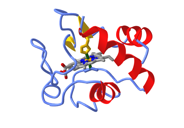) OF YOUR iCn3D MODEL

Figure \(\PageIndex{6}\): [2B4Z]. Click the image for a popup or use this external link: [https://bio.libretexts.org/Learning_..._iCn3Ds_Helena].  (Copyright; author via source).  iCn3D model made by [Helena Prieto]