Models, Simplifying Assumptions and Bounding#
- Page ID
- 8196
\( \newcommand{\vecs}[1]{\overset { \scriptstyle \rightharpoonup} {\mathbf{#1}} } \)
\( \newcommand{\vecd}[1]{\overset{-\!-\!\rightharpoonup}{\vphantom{a}\smash {#1}}} \)
\( \newcommand{\dsum}{\displaystyle\sum\limits} \)
\( \newcommand{\dint}{\displaystyle\int\limits} \)
\( \newcommand{\dlim}{\displaystyle\lim\limits} \)
\( \newcommand{\id}{\mathrm{id}}\) \( \newcommand{\Span}{\mathrm{span}}\)
( \newcommand{\kernel}{\mathrm{null}\,}\) \( \newcommand{\range}{\mathrm{range}\,}\)
\( \newcommand{\RealPart}{\mathrm{Re}}\) \( \newcommand{\ImaginaryPart}{\mathrm{Im}}\)
\( \newcommand{\Argument}{\mathrm{Arg}}\) \( \newcommand{\norm}[1]{\| #1 \|}\)
\( \newcommand{\inner}[2]{\langle #1, #2 \rangle}\)
\( \newcommand{\Span}{\mathrm{span}}\)
\( \newcommand{\id}{\mathrm{id}}\)
\( \newcommand{\Span}{\mathrm{span}}\)
\( \newcommand{\kernel}{\mathrm{null}\,}\)
\( \newcommand{\range}{\mathrm{range}\,}\)
\( \newcommand{\RealPart}{\mathrm{Re}}\)
\( \newcommand{\ImaginaryPart}{\mathrm{Im}}\)
\( \newcommand{\Argument}{\mathrm{Arg}}\)
\( \newcommand{\norm}[1]{\| #1 \|}\)
\( \newcommand{\inner}[2]{\langle #1, #2 \rangle}\)
\( \newcommand{\Span}{\mathrm{span}}\) \( \newcommand{\AA}{\unicode[.8,0]{x212B}}\)
\( \newcommand{\vectorA}[1]{\vec{#1}} % arrow\)
\( \newcommand{\vectorAt}[1]{\vec{\text{#1}}} % arrow\)
\( \newcommand{\vectorB}[1]{\overset { \scriptstyle \rightharpoonup} {\mathbf{#1}} } \)
\( \newcommand{\vectorC}[1]{\textbf{#1}} \)
\( \newcommand{\vectorD}[1]{\overrightarrow{#1}} \)
\( \newcommand{\vectorDt}[1]{\overrightarrow{\text{#1}}} \)
\( \newcommand{\vectE}[1]{\overset{-\!-\!\rightharpoonup}{\vphantom{a}\smash{\mathbf {#1}}}} \)
\( \newcommand{\vecs}[1]{\overset { \scriptstyle \rightharpoonup} {\mathbf{#1}} } \)
\(\newcommand{\longvect}{\overrightarrow}\)
\( \newcommand{\vecd}[1]{\overset{-\!-\!\rightharpoonup}{\vphantom{a}\smash {#1}}} \)
\(\newcommand{\avec}{\mathbf a}\) \(\newcommand{\bvec}{\mathbf b}\) \(\newcommand{\cvec}{\mathbf c}\) \(\newcommand{\dvec}{\mathbf d}\) \(\newcommand{\dtil}{\widetilde{\mathbf d}}\) \(\newcommand{\evec}{\mathbf e}\) \(\newcommand{\fvec}{\mathbf f}\) \(\newcommand{\nvec}{\mathbf n}\) \(\newcommand{\pvec}{\mathbf p}\) \(\newcommand{\qvec}{\mathbf q}\) \(\newcommand{\svec}{\mathbf s}\) \(\newcommand{\tvec}{\mathbf t}\) \(\newcommand{\uvec}{\mathbf u}\) \(\newcommand{\vvec}{\mathbf v}\) \(\newcommand{\wvec}{\mathbf w}\) \(\newcommand{\xvec}{\mathbf x}\) \(\newcommand{\yvec}{\mathbf y}\) \(\newcommand{\zvec}{\mathbf z}\) \(\newcommand{\rvec}{\mathbf r}\) \(\newcommand{\mvec}{\mathbf m}\) \(\newcommand{\zerovec}{\mathbf 0}\) \(\newcommand{\onevec}{\mathbf 1}\) \(\newcommand{\real}{\mathbb R}\) \(\newcommand{\twovec}[2]{\left[\begin{array}{r}#1 \\ #2 \end{array}\right]}\) \(\newcommand{\ctwovec}[2]{\left[\begin{array}{c}#1 \\ #2 \end{array}\right]}\) \(\newcommand{\threevec}[3]{\left[\begin{array}{r}#1 \\ #2 \\ #3 \end{array}\right]}\) \(\newcommand{\cthreevec}[3]{\left[\begin{array}{c}#1 \\ #2 \\ #3 \end{array}\right]}\) \(\newcommand{\fourvec}[4]{\left[\begin{array}{r}#1 \\ #2 \\ #3 \\ #4 \end{array}\right]}\) \(\newcommand{\cfourvec}[4]{\left[\begin{array}{c}#1 \\ #2 \\ #3 \\ #4 \end{array}\right]}\) \(\newcommand{\fivevec}[5]{\left[\begin{array}{r}#1 \\ #2 \\ #3 \\ #4 \\ #5 \\ \end{array}\right]}\) \(\newcommand{\cfivevec}[5]{\left[\begin{array}{c}#1 \\ #2 \\ #3 \\ #4 \\ #5 \\ \end{array}\right]}\) \(\newcommand{\mattwo}[4]{\left[\begin{array}{rr}#1 \amp #2 \\ #3 \amp #4 \\ \end{array}\right]}\) \(\newcommand{\laspan}[1]{\text{Span}\{#1\}}\) \(\newcommand{\bcal}{\cal B}\) \(\newcommand{\ccal}{\cal C}\) \(\newcommand{\scal}{\cal S}\) \(\newcommand{\wcal}{\cal W}\) \(\newcommand{\ecal}{\cal E}\) \(\newcommand{\coords}[2]{\left\{#1\right\}_{#2}}\) \(\newcommand{\gray}[1]{\color{gray}{#1}}\) \(\newcommand{\lgray}[1]{\color{lightgray}{#1}}\) \(\newcommand{\rank}{\operatorname{rank}}\) \(\newcommand{\row}{\text{Row}}\) \(\newcommand{\col}{\text{Col}}\) \(\renewcommand{\row}{\text{Row}}\) \(\newcommand{\nul}{\text{Nul}}\) \(\newcommand{\var}{\text{Var}}\) \(\newcommand{\corr}{\text{corr}}\) \(\newcommand{\len}[1]{\left|#1\right|}\) \(\newcommand{\bbar}{\overline{\bvec}}\) \(\newcommand{\bhat}{\widehat{\bvec}}\) \(\newcommand{\bperp}{\bvec^\perp}\) \(\newcommand{\xhat}{\widehat{\xvec}}\) \(\newcommand{\vhat}{\widehat{\vvec}}\) \(\newcommand{\uhat}{\widehat{\uvec}}\) \(\newcommand{\what}{\widehat{\wvec}}\) \(\newcommand{\Sighat}{\widehat{\Sigma}}\) \(\newcommand{\lt}{<}\) \(\newcommand{\gt}{>}\) \(\newcommand{\amp}{&}\) \(\definecolor{fillinmathshade}{gray}{0.9}\)Models and Simplifying Assumptions
Creating Models of Real Things
Life is complicated. To help us understand what we see around us - in both our everyday lives and in science or engineering - we often construct models. A common aphorism states: All models are wrong, but some are useful. That is, no matter how sophisticated, all models are approximations of something real. While they are not the “real thing” (and are thus wrong), models are useful when they allow us to make predictions about real life that we can use. Models come in a variety of forms that include, but are not limited to:
Types of Models
- Physical models- these are 3D objects that we can touch.
- Drawings - these can be on paper or on the computer and either in 2D or virtual 3D. We mostly look at them.
- Mathematical models - these describe something in real life in mathematical terms. We use these to calculate the behavior of the thing or process we want to understand.
- Verbal or written models - these models are communicated in written or spoken language.
- Mental models - these models are constructed in our minds and we use these to create the other types of models and to understand the things around us.
Simplifying Assumptions
Usually, in science and everyday life alike, simple models are preferred over complex ones. Creating simple models of complex real things requires us to make what are known as simplifying assumptions. As their name implies, simplifying assumptions are assumptions that are included in the model to simplify the analysis as much as possible. When a simplified model no longer predicts behavior of the real thing within acceptable bounds, too many simplifying assumptions have been made. When little predictive value is gained from adding more details to a model, it is likely overly complex. Let’s take a look at different types of models from different disciplines and point out their simplifying assumptions.
An example from physics: A block on a frictionless plane
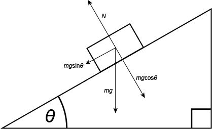
A line drawing that models a block (of any material) sitting on a generic incline plane. In this example some simplifying assumptions are made. For instance, the details of the materials the block and plane are made of are ignored. Often we might also for convenience assume that the plane is frictionless. The simplifying assumptions allow the student to practice thinking about how to balance the forces acting on the block when it is elevated in a gravity field and the surface that it is sitting on is not perpendicular to the gravity vector (mg). This simplifies the math and allows the student to focus on the geometry of the model and how to represent that mathematically. The model, and its simplifying assumptions, might do a reasonably good job of predicting the behavior of an ice cube sliding down an glass incline plane but would likely do a bad job of predicting the behavior of a wet sponge on an incline plane coated with sand paper. The model would be oversimplified for the latter scenario.
Source: Created by Marc T. Facciotti (Own work)
An example from biology: a ribbon diagram of a protein - The transmembrane protein bacteriorhodopsin
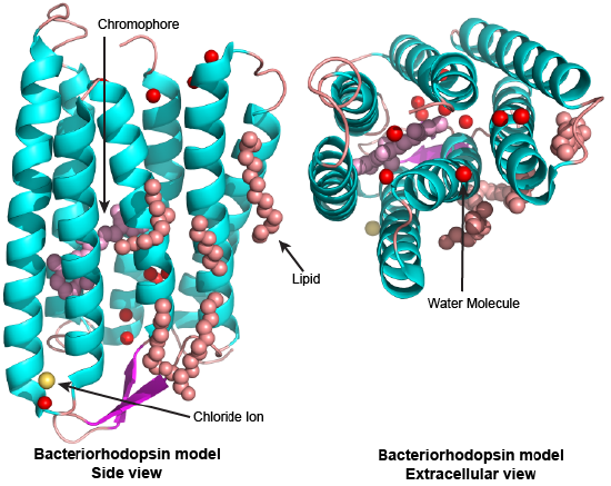
This is a cartoon model of the transmembrane protein bacteriorhodopsin. The protein is represented as a light blue and purple ribbon (the different colors highlight alpha helix and beta sheet, respectively), a chloride ion is represented as a yellow sphere, red spheres represent water molecules, pink balls-and-sticks represent a retinal molecule located on the "inside" of the protein, and orange balls-and-sticks represent other lipid molecules located on the "outside" surface of the protein. The model is displayed in two views. On the left the model is viewed "side on" while on the right it is viewed along its long axis from the extracellular side of the protein (rotated 90 deg out of the page from the view on the left). This model simplifies many of the atomic-level details of the protein. It also fails to represent the dynamics of the protein. The simplifying assumptions mean that the model would not do a good job predicting the time it takes for the protein to do its work or how many protons can be transported across a membrane per second. On the other hand, this model does a very good job of predicting how much space the protein will take up in a cellular membrane, how far into the membrane the retinal sits, or whether certain compounds can reasonably “leak” through the inner channel.
Source: Created by Marc T. Facciotti (own work), University of California, Davis
Derived from PDBID:4FPD
An example from Chemistry: A molecular line model of glucose
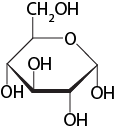
Figure 3: A line drawing of a glucose molecule. By convention, the points where straight lines meet are understood to represent carbon atoms while other atoms are shown explicitly. Given some additional information about the nature of the atoms that are figuratively represented here, this model can be useful for predicting some of the chemical properties of this molecule, including solubility or the potential reactions it might enter into with other molecules. The simplifying assumptions however hide the dynamics of the molecules.
Source: Created by Marc T. Facciotti (Own work)
An example from everyday life: A scale model of a Ferrari
A scale model of a Ferrari. There are many simplifications and most only make this useful for predicting the general shape and relative proportions of the real thing. For instance, this model gives us no predictive power about how well the car drives or how quickly it stops from a speed of 70 km/s.
Source: Created by Marc T. Facciotti (Own work)
Note: Possible discussion
Describe a physical model that you use in everyday life. What does the model simplify from the real thing?
Note: Possible discussion
Describe a drawing that you use in science class to model something real. What does the model simplify from the real thing? What are the advantages and disadvantages of the simplifications?
The spherical cow
The spherical cow is a famous metaphor in physics that make fun of physicists tendencies to create hugely simplified models for very complex things. Numerous jokes are associated with this metaphor and they go something like this:
"Milk production at a dairy farm was low, so the farmer wrote to the local university, asking for help from academia. A multidisciplinary team of professors was assembled, headed by a theoretical physicist, and two weeks of intensive on-site investigation took place. The scholars then returned to the university, notebooks crammed with data, where the task of writing the report was left to the team leader. Shortly thereafter the physicist returned to the farm, saying to the farmer, "I have the solution, but it only works in the case of spherical cows in a vacuum"."
Source: Wikipedia page on Spherical Cow - accessed November 23, 2015.
A cartoon representation of a spherical cow.
Source: https://upload.wikimedia.org/wikiped.../d2/Sphcow.jpg
By Ingrid Kallick (Own work) [GFDL (http://www.gnu.org/copyleft/fdl.html) or CC BY 3.0 (http://creativecommons.org/licenses/by/3.0)], via Wikimedia Commons
The spherical cow is an amusing way to ridicule the process of creating simple models and it is quite likely that you will have your BIS2A instructor invoke the reference to the spherical cow when an overly simplified model of something in biology is being discussed. Be ready for it!
Bounding or Asymptotic Analysis
In BIS2A we use models frequently. Sometimes we also like to imagine or test how well our models actually represent reality and compare that with expectations from what we know to be true for the real life thing. There are many ways to do this depending on how precisely you need to know the behavior of the thing you're trying to model. If you need to know a lot of detail, you create a detailed model. If you're willing to live with less detail, you will create a simpler model. In addition to applying simplifying assumptions, it is often useful to assess your model using a technique we call bounding or asymptotic analysis. The main idea of this technique is to use the model, complete with simplifying assumptions, to understand how the real thing might behave at extreme conditions (e.g. evaluate the model at the minimum and maximum values of a variable). Let’s examine a simple real life example of how this technique works:
Example: Bounding
Problem setup
Imagine that you need to leave Davis, CA and get home to Selma, CA for the weekend. It's 5PM and you told your parents that you'd be home by 6:30. Selma is 200 miles (322 kM) from Davis. You're getting worried that you won't make it home on time. Can you get some estimate of whether it's even possible or if you'll be reheating your dinner in the microwave?
Create Simplified Model and Use of Bounding
You can create a simplified model. In this case you can assume that the road between Davis and Selma is perfectly straight. You also assume that your car has only 2 speeds: 0 mph and 120 mph. These two speeds are the minimum and maximum speeds that you can travel - the bounding values. You can now estimate that even under assumptions of the theoretically "best case" scenario, where you would drive on a perfectly straight road with no obstacles or traffic at maximum speed, you will not make it home on time. At maximum speed you would only cover 180 of the required 200 miles in the 1.5 hours you have.
Interpretation
In this real-life example a simplified model is created. In this case, one very important simplifying assumptions is made: The road is assumed to be straight and free of obstacles or traffic. These assumptions allow you to reasonably assume that you could drive this road at full speed the whole distance. The simplifying assumptions simplified out a lot of what you know is actually there in the real world that would influence the speed you could travel and by extension the time it would take to make the trip. The use of bounding – or calculating the behavior of at the minimum and maximum speeds is a way of making quick predictions about what might happen in the real world.
We will conduct similar analyses in BIS2A.
The importance of knowing key model assumptions
Knowing what simplifying assumptions are made in a model is critical to judging how useful it is for predicting real life and for starting to make a guess about where the model needs improving if it is not sufficiently predictive. In BIS2A you will periodically be asked to create different types of models and to explicitly identify the simplifying assumptions and the impact of those assumptions on the utility and predictive ability of the model. We will also use models together with bounding exercises to try learning something about the potential behavior of a system.


