
4.8: Enzyme Parameters
- Page ID
- 3034

\( \newcommand{\vecs}[1]{\overset { \scriptstyle \rightharpoonup} {\mathbf{#1}} } \)
\( \newcommand{\vecd}[1]{\overset{-\!-\!\rightharpoonup}{\vphantom{a}\smash {#1}}} \)
\( \newcommand{\dsum}{\displaystyle\sum\limits} \)
\( \newcommand{\dint}{\displaystyle\int\limits} \)
\( \newcommand{\dlim}{\displaystyle\lim\limits} \)
\( \newcommand{\id}{\mathrm{id}}\) \( \newcommand{\Span}{\mathrm{span}}\)
( \newcommand{\kernel}{\mathrm{null}\,}\) \( \newcommand{\range}{\mathrm{range}\,}\)
\( \newcommand{\RealPart}{\mathrm{Re}}\) \( \newcommand{\ImaginaryPart}{\mathrm{Im}}\)
\( \newcommand{\Argument}{\mathrm{Arg}}\) \( \newcommand{\norm}[1]{\| #1 \|}\)
\( \newcommand{\inner}[2]{\langle #1, #2 \rangle}\)
\( \newcommand{\Span}{\mathrm{span}}\)
\( \newcommand{\id}{\mathrm{id}}\)
\( \newcommand{\Span}{\mathrm{span}}\)
\( \newcommand{\kernel}{\mathrm{null}\,}\)
\( \newcommand{\range}{\mathrm{range}\,}\)
\( \newcommand{\RealPart}{\mathrm{Re}}\)
\( \newcommand{\ImaginaryPart}{\mathrm{Im}}\)
\( \newcommand{\Argument}{\mathrm{Arg}}\)
\( \newcommand{\norm}[1]{\| #1 \|}\)
\( \newcommand{\inner}[2]{\langle #1, #2 \rangle}\)
\( \newcommand{\Span}{\mathrm{span}}\) \( \newcommand{\AA}{\unicode[.8,0]{x212B}}\)
\( \newcommand{\vectorA}[1]{\vec{#1}} % arrow\)
\( \newcommand{\vectorAt}[1]{\vec{\text{#1}}} % arrow\)
\( \newcommand{\vectorB}[1]{\overset { \scriptstyle \rightharpoonup} {\mathbf{#1}} } \)
\( \newcommand{\vectorC}[1]{\textbf{#1}} \)
\( \newcommand{\vectorD}[1]{\overrightarrow{#1}} \)
\( \newcommand{\vectorDt}[1]{\overrightarrow{\text{#1}}} \)
\( \newcommand{\vectE}[1]{\overset{-\!-\!\rightharpoonup}{\vphantom{a}\smash{\mathbf {#1}}}} \)
\( \newcommand{\vecs}[1]{\overset { \scriptstyle \rightharpoonup} {\mathbf{#1}} } \)
\(\newcommand{\longvect}{\overrightarrow}\)
\( \newcommand{\vecd}[1]{\overset{-\!-\!\rightharpoonup}{\vphantom{a}\smash {#1}}} \)
\(\newcommand{\avec}{\mathbf a}\) \(\newcommand{\bvec}{\mathbf b}\) \(\newcommand{\cvec}{\mathbf c}\) \(\newcommand{\dvec}{\mathbf d}\) \(\newcommand{\dtil}{\widetilde{\mathbf d}}\) \(\newcommand{\evec}{\mathbf e}\) \(\newcommand{\fvec}{\mathbf f}\) \(\newcommand{\nvec}{\mathbf n}\) \(\newcommand{\pvec}{\mathbf p}\) \(\newcommand{\qvec}{\mathbf q}\) \(\newcommand{\svec}{\mathbf s}\) \(\newcommand{\tvec}{\mathbf t}\) \(\newcommand{\uvec}{\mathbf u}\) \(\newcommand{\vvec}{\mathbf v}\) \(\newcommand{\wvec}{\mathbf w}\) \(\newcommand{\xvec}{\mathbf x}\) \(\newcommand{\yvec}{\mathbf y}\) \(\newcommand{\zvec}{\mathbf z}\) \(\newcommand{\rvec}{\mathbf r}\) \(\newcommand{\mvec}{\mathbf m}\) \(\newcommand{\zerovec}{\mathbf 0}\) \(\newcommand{\onevec}{\mathbf 1}\) \(\newcommand{\real}{\mathbb R}\) \(\newcommand{\twovec}[2]{\left[\begin{array}{r}#1 \\ #2 \end{array}\right]}\) \(\newcommand{\ctwovec}[2]{\left[\begin{array}{c}#1 \\ #2 \end{array}\right]}\) \(\newcommand{\threevec}[3]{\left[\begin{array}{r}#1 \\ #2 \\ #3 \end{array}\right]}\) \(\newcommand{\cthreevec}[3]{\left[\begin{array}{c}#1 \\ #2 \\ #3 \end{array}\right]}\) \(\newcommand{\fourvec}[4]{\left[\begin{array}{r}#1 \\ #2 \\ #3 \\ #4 \end{array}\right]}\) \(\newcommand{\cfourvec}[4]{\left[\begin{array}{c}#1 \\ #2 \\ #3 \\ #4 \end{array}\right]}\) \(\newcommand{\fivevec}[5]{\left[\begin{array}{r}#1 \\ #2 \\ #3 \\ #4 \\ #5 \\ \end{array}\right]}\) \(\newcommand{\cfivevec}[5]{\left[\begin{array}{c}#1 \\ #2 \\ #3 \\ #4 \\ #5 \\ \end{array}\right]}\) \(\newcommand{\mattwo}[4]{\left[\begin{array}{rr}#1 \amp #2 \\ #3 \amp #4 \\ \end{array}\right]}\) \(\newcommand{\laspan}[1]{\text{Span}\{#1\}}\) \(\newcommand{\bcal}{\cal B}\) \(\newcommand{\ccal}{\cal C}\) \(\newcommand{\scal}{\cal S}\) \(\newcommand{\wcal}{\cal W}\) \(\newcommand{\ecal}{\cal E}\) \(\newcommand{\coords}[2]{\left\{#1\right\}_{#2}}\) \(\newcommand{\gray}[1]{\color{gray}{#1}}\) \(\newcommand{\lgray}[1]{\color{lightgray}{#1}}\) \(\newcommand{\rank}{\operatorname{rank}}\) \(\newcommand{\row}{\text{Row}}\) \(\newcommand{\col}{\text{Col}}\) \(\renewcommand{\row}{\text{Row}}\) \(\newcommand{\nul}{\text{Nul}}\) \(\newcommand{\var}{\text{Var}}\) \(\newcommand{\corr}{\text{corr}}\) \(\newcommand{\len}[1]{\left|#1\right|}\) \(\newcommand{\bbar}{\overline{\bvec}}\) \(\newcommand{\bhat}{\widehat{\bvec}}\) \(\newcommand{\bperp}{\bvec^\perp}\) \(\newcommand{\xhat}{\widehat{\xvec}}\) \(\newcommand{\vhat}{\widehat{\vvec}}\) \(\newcommand{\uhat}{\widehat{\uvec}}\) \(\newcommand{\what}{\widehat{\wvec}}\) \(\newcommand{\Sighat}{\widehat{\Sigma}}\) \(\newcommand{\lt}{<}\) \(\newcommand{\gt}{>}\) \(\newcommand{\amp}{&}\) \(\definecolor{fillinmathshade}{gray}{0.9}\)Scientists spend a considerable amount of time characterizing enzymes. To understand how they do this and what the characterizations tell us, we must first understand a few parameters. Imagine I wished to study the reaction catalyzed by an enzyme I have just isolated. I would be interested to understand how fast the enzyme works and how much affinity the enzyme has for its substrate(s).
To perform this analysis, I would perform the following experiment. Into 20 different tubes, I would put enzyme buffer (to keep the enzyme stable), the same amount of enzyme, and then a different amount of substrate in each tube, ranging from tiny amounts in the first tubes to very large amounts in the last tubes. I would let the reaction proceed for a fixed, short amount of time and then I would measure the amount of product contained in each tube. For each reaction, I would determine the velocity of the reaction as the concentration of product found in each tube divided by the time. I would then plot the data on a graph using velocity on the Y-axis and the concentration of substrate on the X-axis.
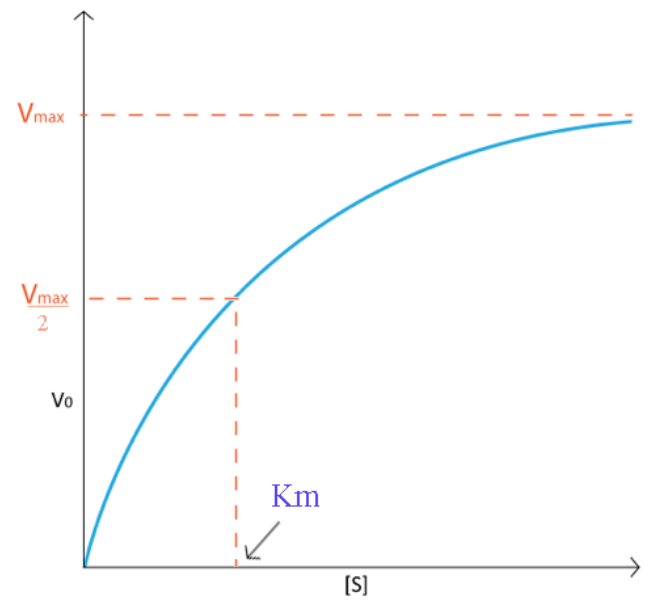
Typically, I would generate a curve like that shown on Figure \(\PageIndex{1}\). Notice how the velocity increase is almost linear in the tubes with the lowest amounts of substrate. This indicates that substrate is limiting and the enzyme converts it into product as soon as it can bind it. As the substrate concentration increases, however, the velocity of the reaction in tubes with higher substrate concentration ceases to increase linearly and instead begins to flatten out, indicating that as the substrate concentration gets higher and higher, the enzyme has a harder time keeping up to convert the substrate to product. What is happening is the enzyme is becoming saturated with substrate at higher concentrations of the latter. Not surprisingly, when the enzyme becomes completely saturated with substrate, it will not have to wait for substrate to diffuse to it and will therefore be operating at maximum velocity.
Turnover Number
On a plot of Velocity versus Substrate Concentration (\(V\) vs. \([S]\)), the maximum velocity (known as \(\text{V}_\text{max}\)) is the value on the Y axis that the curve asymptotically approaches. It should be noted that the value of \(\text{V}_\text{max}\) depends on the amount of enzyme used in a reaction. Double the amount of enzyme, double the \(\text{V}_\text{max}\). If one wanted to compare the velocities of two different enzymes, it would be necessary to use the same amounts of enzyme in the different reactions they catalyze. It is desirable to have a measure of velocity that is independent of enzyme concentration. For this, we define the value \(\text{K}_\text{cat}\), also known as the turnover number. Mathematically,
\[\text{K}_\text{cat} = \dfrac{\text{V}_\text{max}}{ [\text{Enzyme}]} \tag{4.7.1}\]
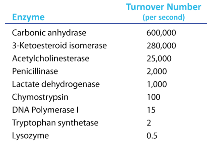
To determine \(\text{K}_\text{cat}\), one must obviously know the \(\text{V}_\text{max}\) at a particular concentration of enzyme, but the beauty of the term is that it is a measure of velocity independent of enzyme concentration, thanks to the term in the denominator. Kcat is thus a constant for an enzyme under given conditions. The units of \(\text{K}_\text{cat}\) are \(\text{time}^{-1}\). An example would be 35/second. This would mean that each molecule of enzyme is catalyzing the formation of 35 molecules of product every second. While that might seem like a high value, there are enzymes known (carbonic anhydrase, for example) that have \(\text{K}_\text{cat}\) values of \(10^6\)/second. This astonishing number illustrates clearly why enzymes seem almost magical in their action.
Michaelis constant
Another parameter of an enzyme that is useful is known as \(\text{K}_\text{M}\), the Michaelis constant. What it measures, in simple terms, is the affinity an enzyme has for its substrate. Affinities of enzymes for substrates vary considerably, so knowing \(\text{K}_\text{M}\) helps us to understand how well an enzyme is suited to the substrate being used. Measurement of KM depends on the measurement of \(V_{max}\). On a \(V\) vs. [S] plot, \(\text{K}_\text{M}\) is determined as the x value that give \(\text{V}_\text{max}/2\). A common mistake students make in describing \(V_{max}\) is saying that \(\text{K}_\text{M} = \text{V}_\text{max}/2\). This is, of course not true. \(\text{K}_\text{M}\) is a substrate concentration and is the amount of substrate it takes for an enzyme to reach \(V_{max}/2\). On the other hand \(V_{max}/2\) is a velocity and is nothing more than that. The value of \(\text{K}_\text{M}\) is inversely related to the affinity of the enzyme for its substrate. High values of \(\text{K}_\text{M}\) correspond to low enzyme affinity for substrate (it takes more substrate to get to \(V_{max}\)). Low \(\text{K}_\text{M}\) values for an enzyme correspond to high affinity for substrate.