2.4.2: Evolution in Populations

Unit 2.4.2 - Evolution in Populations

• Please read and watch the following Learning Resources.
• Reading the material for understanding, and taking notes during videos, will take approximately 1.5 hours.
• Bolded terms are located at the end of the unit in the Glossary. There is also a Unit Summary at the end of the Unit. 
• To navigate to the Unit 2 Glossary, use the Contents menu at the top of the page OR the right arrow on the side of the page.
  • If on a mobile device, use the Contents menu at the top of the page OR the links at the bottom of the page.

Learning Objectives

• Describe how mutations, natural selection, genetic drift, and gene flow can modify the genes in a population.
• Define a population gene pool.
• Explain how the size of the gene pool can affect the evolutionary success of a population.
• Use the Hardy-Weinberg equation to calculate allelic and genotypic frequencies in a population.
• Use the results of a Hardy-Weinberg analysis to determine whether evolution is taking place in a population.

Introduction

Video

This short 3-minute video provides a good introduction to population genetics and its relationship to evolution.
Question after watching: At 2:13, the slide shows four elements that the narrator says are the elements that make up the gene pool. She is incorrect on one count. Which one? And why? Integrate some of the concepts you have learned previously with the ones introduced in this video. Describe how something like a genetic bottleneck might create changes in a population’s gene pool.

The Evolution of Populations

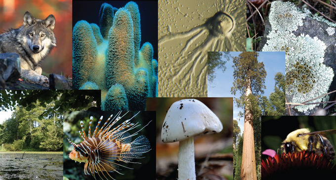
According to evolutionary theory, every organism from humans to beetles to plants to bacteria shares a common ancestor (Figure \(\PageIndex{1}\)). Millions of years of evolutionary pressure caused some species to go extinct while others survived. Earth is filled with more diversity now than at any other point in its history. All life is still connected, however. For example, all organisms are composed of cells and use DNA. The theory of evolution gives us a unifying theory to explain what caused the diversity of species that now exist.

Figure \(\PageIndex{1}\): Evolution has resulted in living things that may be single-celled or complex, multicellular organisms. They may be plants, animals, fungi, bacteria, or Archaea. This diversity results from evolution.

Genetic Variation in Populations

A population is a group of individuals that can all interbreed, often distinguished as a species. These individuals can share genes and pass on combinations of genes to the next generation, containing all of the variation in its gene pool. The process of evolution occurs only in populations and not in individuals. A single individual cannot evolve alone; evolution is the process of changing the gene frequencies within a gene pool. Five forces can cause genetic variation and evolution in a population: mutations, genetic recombination, natural selection, genetic drift, and gene flow. Refresh your understanding of these concepts in Unit 2.2.

Allele Frequencies

A gene for a particular characteristic may have several variations called alleles. These variations code for different traits associated with that characteristic. The allele frequency (or gene frequency) is the rate at which a specific allele exists within a population. Allele frequencies can be expressed as a decimal or as a percent and always add up to 1, or 100 percent, of the total population. The gene pool is the sum of all the alleles of all genes in a population. When calculating the frequency of an allele in a population, remember that for diploid organisms like humans and animals, there are two alleles of each gene in the population.

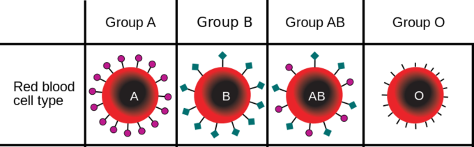
For example, in the ABO blood type system in humans, three alleles (I^A, I^B, or i) determine the particular blood-type of red blood cells (Figure \(\PageIndex{2}\)). Individuals who are phenotypically blood group "A" have the ability to attach certain sugars to the surface of red blood cells. The genotype that confers that ability are I^AI^A or I^Ai. Individuals who are blood group "B" have a different allele of that gene that codes for a protein that adds a different type of sugar on the surface of blood cells. The alleles is labeled I^B, so homozygous I^BI^B or heterozygous I^Bi have that blood type. Individuals who have one allele of each, I^A and I^B can add both sugars on the surface of their blood cells. Finally, people who lack either of these alleles encode an enzyme that cannot add either sugar types and so are blood type "O" and have homozygous alleles ii. 

A diploid organism can only carry two alleles for a particular gene. In human blood type, the combinations are composed of two alleles such as I^AI^A or I^AI^B. Although each organism can only carry two alleles, more than those two alleles may be present in the larger population. In a population of fifty people where all the blood types are represented, there may be more I^A alleles than i alleles. 

Figure \(\PageIndex{2}\): In humans, each blood type corresponds to a combination of two alleles. Human blood types are A, B, AB, and O.

Using the ABO blood type system as an example, the frequency of one of the alleles, for example I^A, is the number of copies of that allele divided by all the copies of the ABO gene in the population, i.e. all the alleles.  In a sample population of humans, the frequency of the I^A allele might be 0.26, which would mean that 26% of the chromosomes in that population carry the I^A allele. If we also know that the frequency of the I^B allele in this population is 0.14, then the frequency of the i allele is 0.6, which we obtain by subtracting all the known allele frequencies from 1 (thus: 1 – 0.26 – 0.14 = 0.6). A change in any of these allele frequencies over time would constitute evolution in the population.

Video

This 4.5-minute video explains how to calculate allelic frequencies in a population. It will also introduce the concept of Hardy-Weinberg equilibrium, which we will explore later in this chapter.
Question after watching: How would you explain the concept of allele frequencies to someone not in your course?

Case of the Hamsters (Part I) - Establishing Alleles

Our case begins with hypothetical species of hamster that carries two alleles for coat color in the population: black which is dominant (B) and grey, which is recessive (b).

Using a Punnett square, if two black hamsters mate that are heterozygous (e.g., Bb) (Table \(\PageIndex{1}\)), we find that

• 25% of their offspring are homozygous for the dominant allele (BB)
• 50% are heterozygous like their parents (Bb)
• 25% are homozygous for the recessive allele (bb) and thus, unlike their parents, express the recessive phenotype.

Note

Find a refresher on Punnett squares here: Punnett Squares

This is what Mendel found when he crossed monohybrids. It occurs because meiosis separates the two alleles of each heterozygous parent so that 50% of the gametes will carry one allele and 50% the other and when the gametes are brought together at random, each B (or b)-carrying egg will have a 1 in 2 probability of being fertilized by a sperm carrying B (or b).

Table \(\PageIndex{1}\). Results of the random union of the two gametes produced by two individuals, each heterozygous for a given trait. As a result of meiosis, half the gametes produced by each parent will carry allele B; the other half allele b.
	0.5 B	0.5 b
0.5 B	0.25 BB	0.25 Bb
0.5 b	0.25 Bb	0.25 bb

However, the frequency of two alleles in an entire population of organisms is unlikely to be exactly the same. We will return to this case in a moment.

The Hardy-Weinberg Principle: A Theory of Population Evolution

Theoretical Background

In the early twentieth century, English mathematician Godfrey Hardy and German physician Wilhelm Weinberg stated the principle of equilibrium to describe the population's genetic makeup. The theory, which later became known as the Hardy-Weinberg principle of equilibrium, states that a population’s allele and genotype frequencies are inherently stable— unless some kind of evolutionary force is acting upon the population, neither the allele nor the genotypic frequencies would change. 

Ultimately, the Hardy-Weinberg principle models a population without evolution under the following conditions:

1. no mutations
2. no immigration/emigration
3. no natural selection
4. only random matings
5. a large population

In theory, if a population is at equilibrium—that is, there are no evolutionary forces such as natural selection, mutation, etc. acting upon it—generation after generation would have the same gene pool and genetic structure, and the allele frequencies would stay the same over time. This is because all of the alleles would have an equal chance of being passed to the next generation and the ratios would remain constant.

Of course, even Hardy and Weinberg recognized that no natural population is immune to evolution. Evolution involves changes in the gene pool. Populations in nature are constantly changing in genetic makeup due to drift, mutation, possibly migration, and selection.

Note: The Hardy-Weinberg Principle

So long as certain conditions are met (discussed below), allele frequencies and genotype ratios in a randomly-breeding population remain constant from generation to generation. This is known as the Hardy-Weinberg Principle.

As a result, the only way to determine the exact distribution of phenotypes in a population is to go out and count them. A population in Hardy-Weinberg equilibrium shows no change. What the law tells us is that populations are able to maintain a reservoir of variability so that if future conditions require it, the gene pool can change. If the frequencies of alleles or genotypes deviate from the value expected from the Hardy-Weinberg equation, then the population is evolving.

When populations are in the Hardy-Weinberg equilibrium, the allelic frequency is stable from generation to generation and the distribution of alleles can be determined. If the allelic frequency measured in the field differs from the predicted value, scientists can make inferences about what evolutionary forces are at play. However, what ultimately interests most biologists is not the frequencies of different alleles, but the frequencies of the resulting genotypes, from which scientists can surmise phenotype distribution.

Video

This 11-minute Crash Course video provides an overview of population genetics in a humorous manner.
Questions after watching: In this video, the narrator says there are five ways to alter the gene pool of a population. Explain how this could be. What’s another way to say that a population is in Hardy-Weinberg equilibrium?

Applying Hardy-Weinberg

While no population can satisfy those conditions, the principle offers a useful model against which to compare real population changes. The genetic variation of natural populations is constantly changing from genetic drift, gene flow, mutation, migration, and natural selection. Population genetics is the study of the distributions and changes of allele frequency in a population. In population genetics, evolution is defined as a change in the frequency of an allele in a population.

The Hardy-Weinberg principle gives scientists a mathematical baseline of a non-evolving population to which they can compare observable populations in the field or laboratory to determine whether they are evolving. If scientists record allele frequencies over time and then calculate the expected frequencies based on Hardy-Weinberg values, then scientists can detect when a population deviates from HW expectations and therefore confirm that the population is evolving. The Hardy-Weinberg principle states that a population’s allele and genotype frequencies will remain constant in the absence of evolutionary mechanisms. Note that this conclusion does not inform the researcher as to which mechanism of allelic frequency change is at play, only that allelic frequencies are changing (i.e. that evolution is occurring).

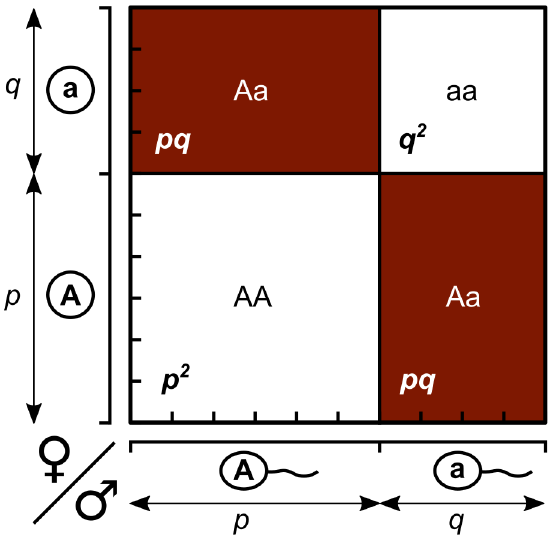
Working under this theory, population geneticists represent different alleles as different variables in their mathematical models (Figure \(\PageIndex{3}\)). The variable \(p\), for example, represents the frequency of a particular allele, say A for the trait of tall plants in Mendel’s peas, while the variable \(q\) represents the frequency of alleles that confer the short plant trait, a. If these are the only two possible alleles for a given locus in the population, then \(p\) + \(q\) = 1. In other words, all the \(p\) alleles and all the \(q\) alleles comprise all of the alleles for that locus in the population.

If we observe the phenotype, we can know only the homozygous recessive allele's genotype. The Hardy-Weinberg calculations provide an estimate of the remaining genotypes. Since each individual carries two alleles per gene, if we know the allele frequencies (\(p\) and \(q\)), predicting the genotypes' frequencies is a simple mathematical calculation to determine the probability of obtaining these genotypes if we draw two alleles at random from the gene pool, as we will see below.

Figure \(\PageIndex{3}\): Hardy-Weinberg and the Punnett Square. (CC0 1.0)

Calculating Gene Pools and Genotype Frequencies

Gene pools

The total number of genes in a population is its gene pool.

• Let \(p\) represent the frequency of the dominant allele in the gene pool and \(q\) the frequency of the recessive allele in the gene pool.
• Because p and q together equal all of the alleles in the gene pool, \(p + q = 1\)

Genotype frequencies

• Homozygous dominant individuals have two \(p\) alleles. Their genotype frequency can be determined by \(p\) x \(p\) or \(p^2\).
• Similarly, homozygous recessive individuals have two \(q\) alleles. Their genotype frequency can be determined by \(q\) x \(q\) or \(q^2\)
• Heterozygous individuals are \(2pq\). Their genotype frequency can be determined by 2 x \(p\) x \(q\) or \(2pq\).  [There are two possible types of heterozygous unions: pq and qp. Therefore, we calculate 2 x p x q]  
• Because \(p^2\), \(q^2\), and \(2pq\) together equal all of the genotypes in a population, \(p^2\) + \(2pq\) + \(q^2\) = 1

If any one of the variables above is known, the allele frequency or genotype frequencies can be calculated. We will revisit our case study below to see how these equations are put into practice by scientists to understand whether evolution is occurring in a population.

Video

This 11-minute video describes how to calculate allele and gene pool frequencies with the Hardy-Weinberg equations. Examples and practice equations are given below. 

Case of the Hamsters (Part II) - Calculating Allele and Genotype Frequency

The frequency of two alleles in an entire population of organisms is unlikely to be exactly the same as we saw in the Punnett square of Part 1. However, from a given genotype (or recessive phenotypes since that genotype is known), we can infer the frequencies of the alleles in a population.

Since each diploid individual carries two alleles per gene, we can predict the frequencies of these genotypes using a probability matrix Table \(\PageIndex{2}\). If two alleles are drawn at random from the gene pool, we can determine the probability of each genotype. We are now calculating percentages based on overall populations (not individual pairings like a Punnett square). In this type of probability matrix, all of the alleles that can mix in a population to produce the next generation are represented.

1. Revisiting our hypothetical case of a population of hamsters, for the purposes of example, we will establish that 80% of all the gametes in the population carry a dominant allele for black coat (B) and 20% carry the recessive allele for gray coat (b). So, \(p\) = 0.8 and \(q\) = 0.2.
2. We can now use those two values to calculate the genotype frequencies where \(p^2\) = 0.64 and \(q^2\) = 0.04
3. The equation above states \(p^2\) + \(2pq\) + \(q^2\) = 1. We have calculated \(p^2\) and \(q^2\) but need to now solve for \(2pq\).
4. We can determine from our calculations that 0.64 + \(2pq\) + 0.04 = 1
5. From there 0.64 + 0.04 + \(2pq\) = 1
6. And 0.68 + \(2pq\) = 1
7. So, \(2pq\) = 1 - 0.68 = 0.32 or 32%

Therefore, in this case, the random union of these allele frequencies will produce a generation:

• 64% homozygous for BB
• 32% Bb heterozygotes 
• 4% homozygous (bb) for gray coat 

So 96% of the next generation will have black coats; only 4% gray coats. If you notice, this is the same phenotype ratio as the initial population. No change has occurred, which is explained in more detail below.

Table \(\PageIndex{2}\). Results of random union of the gametes produced by an entire population with a gene pool containing 80% B and 20% b.
	0.8 B	0.2 b
0.8 B	0.64 BB	0.16 Bb
0.2 b	0.16 Bb	0.04 bb

Hardy-Weinberg and Selection Pressures

Natural selection affects allele and genotype frequency. If an allele confers a phenotype that enables an individual to better survive or have more offspring, the frequency of that allele will increase because the individual carrying these alleles will be effective at transferring them into the next generation. Because many of those offspring will also carry the beneficial allele and, therefore, the phenotype, they will have more offspring of their own that also carry the allele. Over time, the allele will spread throughout the population and may become fixed: every individual in the population carries the allele. If an allele is dominant but detrimental, it may be swiftly eliminated from the gene pool when the individual with the allele does not reproduce. However, a detrimental recessive allele can linger for generations in a population, hidden by the dominant allele in heterozygotes. In such cases, the only individuals to be eliminated from the population are those unlucky enough to inherit two copies of such an allele.

So, will deleterious alleles eventually disappear? No. Let's see why using our case study.

Imagine that the grey coat color carries with it some sore of negative selection pressure. If we calculate the allele frequencies, using our genotype frequencies from Table \(\PageIndex{2}\) above, we can recalculate how much of the population carries the dominant allele and what percentage carries the recessive allele.

• All the gametes formed by BB hamsters will contain allele B (0.64) as will one-half the gametes formed by heterozygous (Bb) hamsters (0.32/2).
  • So, 80% (0.64 + (0.32*1/2)) of the pool of gametes formed by this generation will contain B.
• All the gametes of the gray (bb) hamsters (4%) will contain b (0.04) but one-half of the gametes of the heterozygous hamsters will as well (0.32/2).
  • So 20% (0.04 + (0.32*1/2)) of the gametes will contain b.

What we find from this analysis is that in the parental generation, 80% of the alleles were B and 20% of the alleles were b. The organisms of that population mated and produced generation 2. This was a random sampling event of the alleles in the parental gene pool. In the generation 2 alleles, we find that 80% of the alleles are B and 20% are b. This is identical to the parental allelic frequency.

The proportion of allele b in the population has remained the same from the parent generation. The heterozygous hamsters ensure that each generation will contain 4% gray hamsters. Recessive genes do not tend to be lost from a population no matter how small their representation. If recessive alleles were continually tending to disappear, the population would soon become homozygous. Under Hardy-Weinberg conditions, genes that have no present selective value will nonetheless be retained.

If an allele confers a phenotype that enables an individual to better survive or have more offspring, the frequency of that allele will increase because the individual carrying these alleles will be effective at transferring them into the next generation. Because many of those offspring will also carry the beneficial allele and, therefore, the phenotype, they will have more offspring of their own that also carry the allele. Over time, the allele will spread throughout the population and may become fixed: every individual in the population carries the allele. If an allele is dominant but detrimental, it may be swiftly eliminated from the gene pool when the individual with the allele does not reproduce. However, a detrimental recessive allele can linger for generations in a population, hidden by the dominant allele in heterozygotes. In such cases, the only individuals to be eliminated from the population are those unlucky enough to inherit two copies of such an allele.

Optional Activity \(\PageIndex{1}\)

In the Punnett square in Figure \(\PageIndex{4}\), an individual pea plant could be pp (YY), and thus produce yellow peas; pq (Yy), also yellow; or qq (yy), and thus produce green peas. If 9% of the overall plants in a population produce green peas, what percentage of pea plants are heterozygous for pea color?

Answer (Click here)

According to the Hardy-Weinberg principle, the variable p represents the frequency of a particular allele, usually a dominant one. For example, assume that p represents the frequency of the dominant allele, Y, for yellow pea pods. The variable q represents the frequency of the recessive allele, y, for green pea pods. If p and q are the only two possible alleles for this characteristic, then the sum of the frequencies must add up to 1, or 100 percent. We can also write this as p + q = 1. If the frequency of the Y allele in the population is 0.6, then we know that the frequency of the y allele is 0.4.

In the example, our three genotype possibilities are: pp (YY), producing yellow peas; pq (Yy), also yellow; or qq (yy), producing green peas. The frequency of homozygous dominant individuals is p²; the frequency of heterozygous individuals is 2pq; and the frequency of homozygous recessive individuals is q². If p and q are the only two possible alleles for a given trait in the population, these genotype frequencies will sum to one: p² + 2pq + q² = 1.

In our example, the possible genotypes are homozygous dominant (YY), heterozygous (Yy), and homozygous recessive (yy). If we can only observe the phenotypes in the population, then we know only the recessive phenotype (yy). For example, in a garden of 100 pea plants, 86 might have yellow peas and 16 have green peas. We do not know how many are homozygous dominant (Yy) or heterozygous (Yy), but we do know that 16 of them are homozygous recessive (yy).

Therefore, by knowing the recessive phenotype and, thereby, the frequency of that genotype (16 out of 100 individuals or 0.16), we can calculate the number of other genotypes.

1. If q² represents the frequency of homozygous recessive plants, then q² = 0.16.
2. Therefore, q = 0.4 (the square root of 0.16 is 0.4...we cannot have a negative number when working with allele frequencies).
3. Because p + q = 1 and q = 0.4, then 1 – 0.4 = p.
4. p = 0.6.
5. The frequency of homozygous dominant plants (p²) is (0.6)² = 0.36. So, out of 100 individuals, there are 36 homozygous dominant (YY) plants.
6. The frequency of heterozygous plants (2pq) is 2(0.6)(0.4) = 0.48. Therefore, 48 out of 100 plants are heterozygous yellow (Yy).

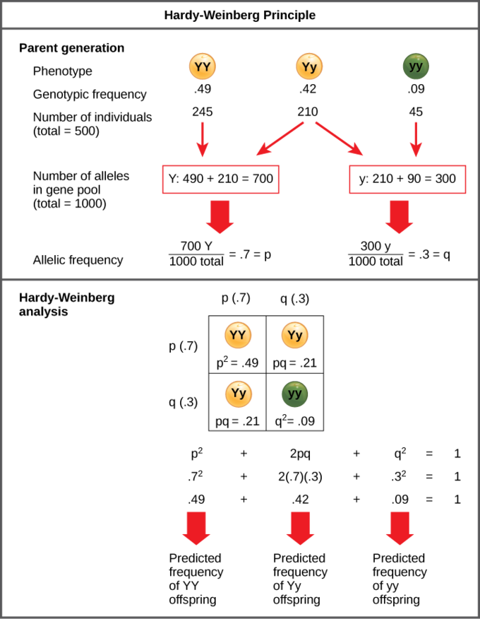
Figure \(\PageIndex{4}\): Predicted frequencies of alleles and genotypes of a population with 9% green peas.

Optional Activity \(\PageIndex{2}\)

In plants, violet flower color (V) is dominant over white (v). If q = 0.2 in a population of 500 plants, how many individuals would you expect to be homozygous dominant (VV), heterozygous (Vv), and homozygous recessive (vv)? How many plants would you expect to have violet flowers, and how many would have white flowers?

Answer

Remember that p indicates the frequency of the dominant allele (V) and q indicates the frequency of the recessive allele (v). It is easier to begin with the recessive allele. 

In this population, if q = 0.2, then q² = 0.04. We know that q² is the frequency of homozygous recessive individuals, so 0.04 x 500 total plants (the overall population) = 20. Therefore, 20 plants would be expected to be homozygous recessive (white).  

For the dominant allele, p, we need to use the formula p + q = 1. Since q = 0.2, we can calculate p + 0.2 = 1. From there, we get p = 1 - 0.2 so p = 0.8. 

If p = 0.8, then p2 = 0.64. We know that p2 is the frequency of homozygous dominant individuals, so 0.64 x 500 total plants (the overall population) = 320. Therefore, 320 plants are expected to be homozygous dominant (violet).

To complete the problem, we calculate 2pq, or the frequency of heterozygous individuals. So, 2 x 0.8 x 0.2 = 0.32. We will then take and calculate 0.32 x 500 to get 160. Therefore, 160 plants are expected to be heterozygous (violet).

  

Optional Resource

Find an additional Hardy-Weinberg problem to solve, with a solution and walk-through, here.

When the Hardy-Weinberg Law Fails

To see what forces lead to evolutionary change, we must examine the circumstances in which the Hardy-Weinberg law may fail to apply. In any of these cases (which is the reality of the natural world), evolution is occurring. There are five:

1. Mutation

The frequency of gene B and its allele b will not remain in Hardy-Weinberg equilibrium if the rate of mutation of B -> b (or vice versa) changes, or if a new allele B^o comes to be. By itself, this type of mutation probably plays only a minor role in evolution; the rates are simply too low. However, gene (and whole genome) duplication - a form of mutation - probably has played a major role in evolution. In any case, evolution depends on mutations because this is the only way that new alleles are created. After being shuffled in various combinations with the rest of the gene pool, these provide the raw material on which natural selection can act.

2. Gene Flow

Many species are made up of local populations whose members tend to breed within the group. Each local population can develop a gene pool distinct from that of other local populations. However, members of one population may breed with occasional immigrants from an adjacent population of the same species. This can introduce new genes or alter existing gene frequencies in the residents. Whether within a species or between species, gene flow increases the variability of the gene pool.

3. Genetic Drift

Genetic drift is the evolution that happens when there is no selective advantage for the alleles that grow in frequency. That growth is due to chance events. For example, if a rock falls on a population of beetles that have green and red alleles and kills more of those individuals with the red allele, the gene frequency for this gene will change, but it was not adaptive. It just happened due to chance events. The smaller a population, the more susceptible it is to mechanisms such as genetic drift. Random events that alter allele frequencies will have a much larger effect when the gene pool is small. 

If the population is small, Hardy-Weinberg may be violated. Chance, including abiotic impacts, alone may eliminate certain members out of proportion to their numbers in the population. In such cases, the frequency of an allele may begin to drift toward higher or lower values. Ultimately, the allele may represent 100% of the gene pool or, just as likely, disappear from it. Drift produces evolutionary change, but there is no guarantee that the new population will be more fit than the original one. Evolution by drift is aimless, not adaptive.

4. Nonrandom Mating

One of the cornerstones of the Hardy-Weinberg equilibrium is that mating in the population must be random. If individuals (usually females) are choosy in their selection of mates, the gene frequencies may become altered. 

Nonrandom mating seems to be quite common. Breeding territories, courtship displays, "pecking orders" can all lead to it. In each case, certain individuals do not get to make their proportionate contribution to the next generation. If some males reproduce more than others, then more of their genes are represented in the next generation.

5. Natural Selection

If individuals having certain genes are better able to produce mature offspring than those without them, the frequency of those genes will increase in the next generation. This is simply expressing Darwin's natural selection in terms of alterations in the gene pool. Natural selection results from differential mortality (some individuals survive longer than others) and/or differential fecundity (some individuals have more offspring than others). Ultimately, this causes the sampling of one generation’s gene pool to be skewed; the next generation’s gene pool is different from the first. Not every allele has an equal chance of being passed on to the next generation.

Video

This 4-minute video explains what the Hardy-Weinberg equilibrium is and why finding a population that does not conform to HW expectations tells you that the population is in the process of evolving with regard to one trait.
Question after watching: The HW principle is defined using mathematical terms. Based on what you now know about the HW principle, what is being quantified and monitored in the HW principle to assess whether a population is evolving?