22.2: Diversity Indices

Last updated
Save as PDF

Page ID: 84119

\( \newcommand{\vecs}[1]{\overset { \scriptstyle \rightharpoonup} {\mathbf{#1}} } \) \( \newcommand{\vecd}[1]{\overset{-\!-\!\rightharpoonup}{\vphantom{a}\smash {#1}}} \)\(\newcommand{\id}{\mathrm{id}}\) \( \newcommand{\Span}{\mathrm{span}}\) \( \newcommand{\kernel}{\mathrm{null}\,}\) \( \newcommand{\range}{\mathrm{range}\,}\) \( \newcommand{\RealPart}{\mathrm{Re}}\) \( \newcommand{\ImaginaryPart}{\mathrm{Im}}\) \( \newcommand{\Argument}{\mathrm{Arg}}\) \( \newcommand{\norm}[1]{\| #1 \|}\) \( \newcommand{\inner}[2]{\langle #1, #2 \rangle}\) \( \newcommand{\Span}{\mathrm{span}}\) \(\newcommand{\id}{\mathrm{id}}\) \( \newcommand{\Span}{\mathrm{span}}\) \( \newcommand{\kernel}{\mathrm{null}\,}\) \( \newcommand{\range}{\mathrm{range}\,}\) \( \newcommand{\RealPart}{\mathrm{Re}}\) \( \newcommand{\ImaginaryPart}{\mathrm{Im}}\) \( \newcommand{\Argument}{\mathrm{Arg}}\) \( \newcommand{\norm}[1]{\| #1 \|}\) \( \newcommand{\inner}[2]{\langle #1, #2 \rangle}\) \( \newcommand{\Span}{\mathrm{span}}\)\(\newcommand{\AA}{\unicode[.8,0]{x212B}}\)

Diversity Indices

A diversity index is a quantitative measure that reflects how many different types (such as species) there are in a dataset (a community). These indices are statistical representations of biodiversity in different aspects (richness, evenness, and dominance). When diversity indices are used in ecology, the types of interest are usually species, but they can also be other categories, such as genera, families, functional types, or haplotypes. The entities of interest are usually individual plants or animals, and the measure of abundance can be, for example, number of individuals, biomass or coverage.

Richness simply quantifies how many different types the dataset of interest contains. For example, species richness (usually noted S) of a dataset is the number of species in the corresponding species list. Richness is a simple measure, so it has been a popular diversity index in ecology, where abundance data are often not available for the datasets of interest.

Although species richness (denoted S) is often used as a measure of biodiversity, of more interest to ecologists and conservation biologists are diversity indices that include both species richness and measures of abundance. This is because richness alone does not account for evenness across species. In example 22.2.1 below, both lakes have the same richness, but Lake B is more diverse because abundance is spread more evenly across the species present.

Many different indices of diversity are used by scientists, but below we cover the most widely used.

Simpson’s Index

Simpson (1949) developed an index of diversity which is a measure of probability--the less diversity, the greater the probability that two randomly selected individuals will be the same species. In the absence of diversity (1 species), the probability that two individuals randomly selected will be the same is 1. Simpson's Index is calculated as follows:

\[D=\sum_{i=1}^{S}\left(\frac{n_{i}}{N}\right)^{2}\]

where n_iis the number of individuals in species i, N = total number of individuals of all species, and n_i/N = p_i (proportion of individuals of species i), and S = species richness.

The value of Simpson’s D ranges from 0 to 1, with 0 representing infinite diversity and 1 representing no diversity, so the larger the value of D, the lower the diversity. For this reason, Simpson’s index is often as its complement (1-D). Simpson's Dominance Index is the inverse of the Simpson's Index (1/D).

Shannon-Weiner Index

Another widely used index of diversity that also considers both species richness and evenness is the Shannon-Weiner Diversity Index, originally proposed by Claude Shannon in 1948. It is also known as Shannon's diversity index. The index is related to the concept of uncertainty. If for example, a community has very low diversity, we can be fairly certain of the identity of an organism we might choose by random (high certainty or low uncertainty). If a community is highly diverse and we choose an organism by random, we have a greater uncertainty of which species we will choose (low certainty or high uncertainty).

\[H=-\sum_{i=1}^{S} p_{i} * \ln p_{i}\]

where p_i = proportion of individuals of species i, and ln is the natural logarithm, and S = species richness.

The value of H ranges from 0 to H_max_.H_max is different for each community and depends on species richness. (Note: Shannon-Weiner is often denoted H' ).

Evenness Index

Species evenness refers to how close in numbers each species in an environment is. So if there are 40 foxes and 1000 dogs, the community is not very even. But if there are 40 foxes and 42 dogs, the community is quite even. The evenness of a community can be represented by Pielou's evenness index (Pielou 1966):

\[J=\frac{H}{H_{\max }}\]

The value of J ranges from 0 to 1. Higher values indicate higher levels of evenness. At maximum evenness, J = 1.

J and D can be used as measures of species dominance (the opposite of diversity) in a community. Low J indicates that 1 or few species dominate the community.

Example \(\PageIndex{1}\)

Calculate Simpson's Index, Shannon-Weiner Index, and the Evenness Index for waterbirds on two lakes: Lake A, and Lake B. There are 5 species and 25 individuals on both lakes, but are they equally diverse?

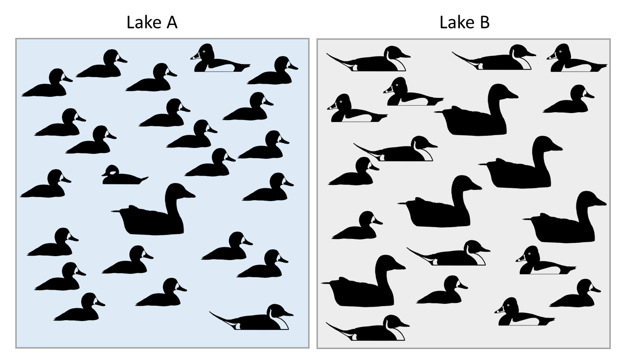
Two lakes both have 25 total birds, with five different species in each lake. In Lake A, three of the bird species only have one bird from each species, while the other 21 birds are from the fifth species. In Lake A, each of the five species has five individuals from each species.

Figure \(\PageIndex{1}\): Though both Lakes A and B have the same amount of birds and the same number of different species, their diversity is different.

Here are the solutions:

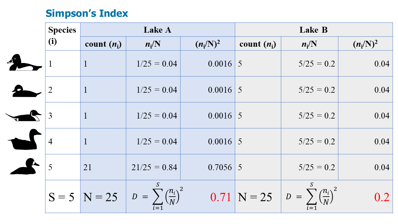
Simpson's Index is used to calculate D for Lakes A and B. For Lake A, D = 0.71 and for Lake B, D = 0.2.

Figure \(\PageIndex{2}\): The three blue columns show the steps to calculate D for Lake A, while the three gray columns show the steps to calculate D for Lake B. Though the S and N values are the same for both lakes, the proportion of each species in the lakes results in different D values.

Note that Simpson's Index is often expressed (1-D), so the final answers are 0.29 and 0.8. This makes more intuitive sense: a higher D is more diverse--which is Lake B because it is less dominated by one species.

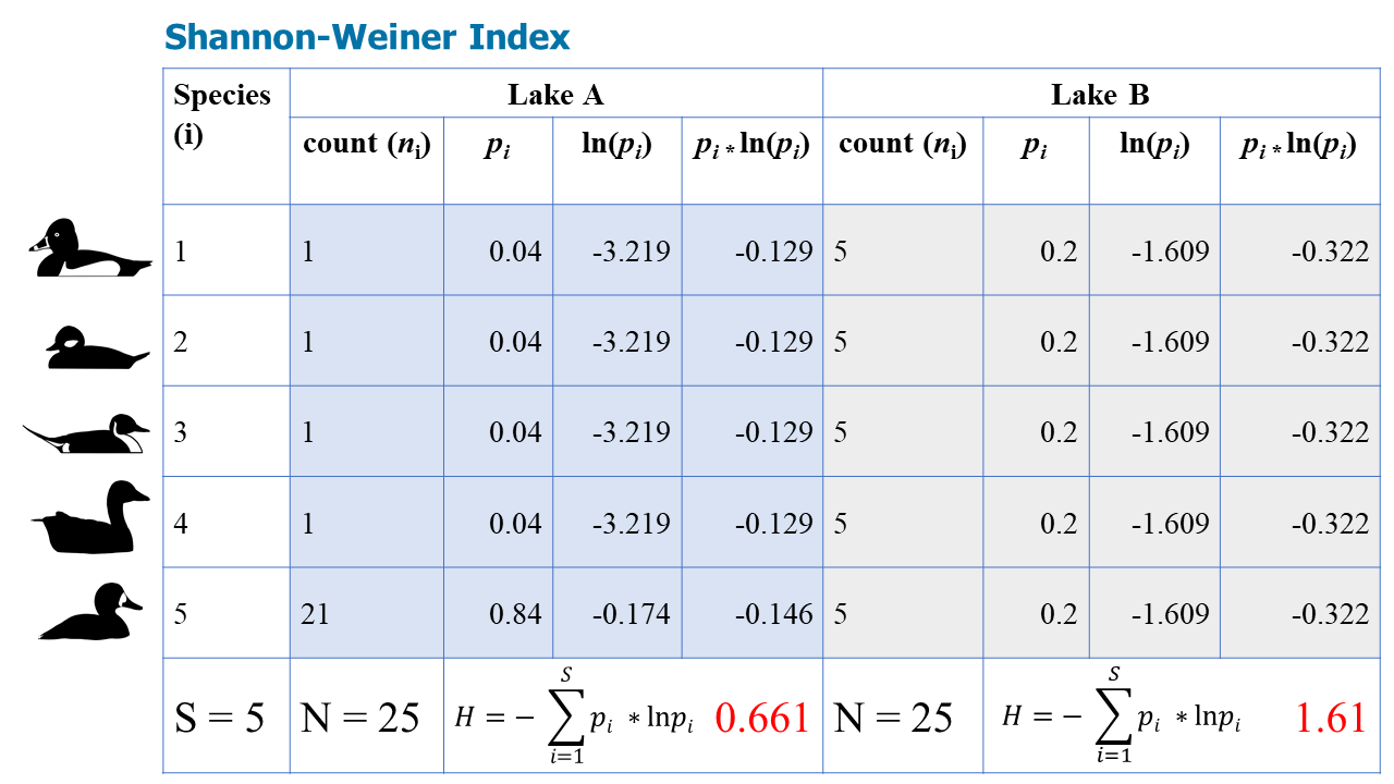
The Shannon-Weiner Index is used to calculate H for Lakes A and B. For Lake A, H = 0.661 and for Lake B, H = 1.61.

Figure \(\PageIndex{3}\): The four blue columns show the steps to calculate H for Lake A, while the four gray columns show the steps to calculate H for Lake B.

Again, according to the Shannon-Weiner Index, Lake B is more diverse.

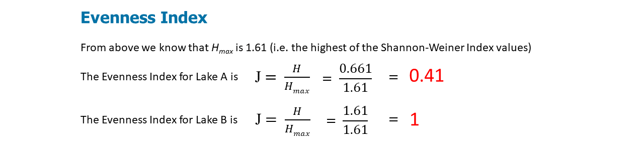
Species evenness (J) is calculated for Lakes A and B. For Lake A, J = 0.41. For Lake B, J = 1.

Figure \(\PageIndex{4}\): J calculates the species evenness for Lakes A and B using the Shannon-Weiner Index calculations.

Conclusion

By all three measures, Lake B is more diverse, despite the fact that the two lakes have identical species richness.

Biodiversity at different scales- Alpha, Beta, and Gamma

Biologists have developed three quantitative measures of species diversity as a means of measuring and comparing species diversity:

Alpha diversity (or species richness), the most commonly referenced measure of species diversity, refers to the total number of species found in a particular biological community, such as a lake or a forest. Bwindi Forest in Uganda, with an estimated 350 bird species, has one of the highest alpha diversities of all African ecosystems.
Gamma diversity describes the total number of species that occur across an entire region, such as a mountain range or continent, that includes many ecosystems. The Albertine Rift, which includes Bwindi Forest, has more than 1,074 species of birds, a very high gamma diversity for such a small region.
Beta diversity connects alpha and gamma diversity. It describes the rate at which species composition changes across a region. For example, if every wetland in a region was inhabited by a similar suite of plant species, then the region would have low beta diversity; in contrast, if several wetlands in a region had plants communities that were distinct and had little overlap with one another, the region would have high beta diversity. Beta diversity is calculated as gamma diversity divided by alpha diversity. The beta diversity for forest birds of the Albertine Rift is about 3.0, if each ecosystem in the area has about the same number of species as Bwindi Forest.

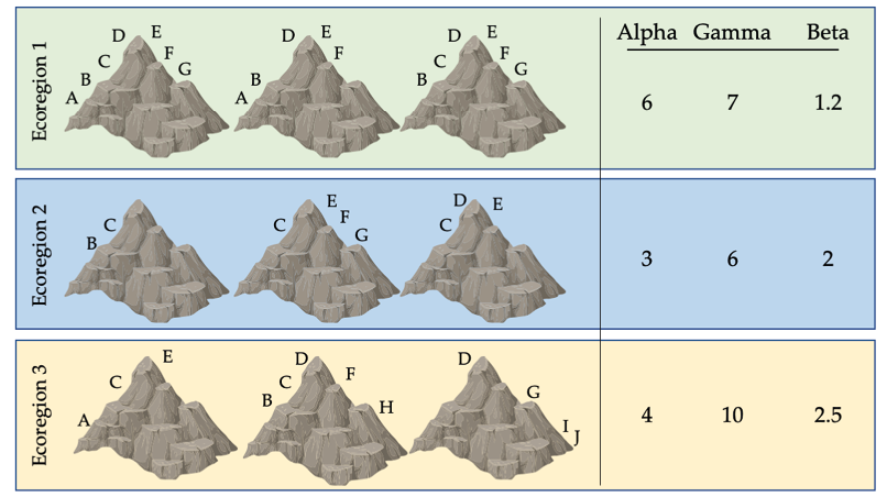
Three mountains in three different ecoregions have species A through J. For ecoregion 1, alpha is 6, gamma is 7, and beta is 1.2. For ecoregion 2, alpha is 3, gamma is 6, and beta is 2. For ecoregion 3, alpha is 4, gamma is 10, and beta is 2.5.

Figure \(\PageIndex{5}\): Biodiversity indices for nine mountain peaks across three ecoregions. Each symbol represents a different species; some species have populations on only one peak, while others are found on two or more peaks. The variation in species richness on each peak results in different alpha, gamma, and beta diversity values for each ecoregion. This variation has implications for how we divide limited resources to maximise protection. If only one ecoregion can be protected, ecoregion 3 may be a good choice because it has high gamma (total) diversity. However, if only one peak can be protected, should a peak in ecoregion 1 (with many widespread species) or ecoregion 3 (with several unique, range-restricted species) be protected? After Primack, 2012, CC BY 4.0.

It is important to note that alpha, beta, and gamma diversity describe only part of what is meant by biodiversity. For example, none of these three terms completely account for genetic diversity, which allows species to adapt as conditions change. It also neglects the importance of ecosystem diversity, which results from the collective response of species to their dynamic environment. However, these diversity measures are useful for comparing different regions, and identifying locations with high concentrations of native species that should be protected.

References

Pielou, E.C. (1966). The measurement of diversity in different types of biological collections. Journal of Theoretical Biology, 13, pp. 131–144. doi:10.1016/0022-5193(66)90013-0.

Simpson, E.H. (1949). Measurement of diversity. Nature, 163, pp. 688. doi:10.1038/163688a0

Shannon, C.E. (1948). A mathematical theory of communication. The Bell System Technical Journal, 27, pp. 379-423.
https://doi.org/10.1002/j.1538-7305.1948.tb01338.x

Contributors and Attributions

Written and curated by A. Wilson and N. Gownaris (Gettysburg College) with material from the following open-access sources: