45.2B: Logistic Population Growth

Learning Objectives

• Describe logistic growth of a population size

Exponential growth is possible only when infinite natural resources are available; this is not the case in the real world. Charles Darwin recognized this fact in his description of the “struggle for existence,” which states that individuals will compete (with members of their own or other species ) for limited resources. The successful ones will survive to pass on their own characteristics and traits (which we know now are transferred by genes) to the next generation at a greater rate: a process known as natural selection. To model the reality of limited resources, population ecologists developed the logistic growth model.

Carrying Capacity and the Logistic Model

In the real world, with its limited resources, exponential growth cannot continue indefinitely. Exponential growth may occur in environments where there are few individuals and plentiful resources, but when the number of individuals becomes large enough, resources will be depleted, slowing the growth rate. Eventually, the growth rate will plateau or level off. This population size, which represents the maximum population size that a particular environment can support, is called the carrying capacity, or \(K\).

The formula we use to calculate logistic growth adds the carrying capacity as a moderating force in the growth rate. The expression “K – N” is indicative of how many individuals may be added to a population at a given stage, and “K – N” divided by “K” is the fraction of the carrying capacity available for further growth. Thus, the exponential growth model is restricted by this factor to generate the logistic growth equation:

\[ \begin{align*} \dfrac{dN}{dT} &=r_{max} \dfrac{dN}{dT} \\[4pt] &=r_{max} \times N \times (\dfrac{K- N}{K}) \dfrac{dN}{dT} \\[4pt] &=rmax∗(dN/dT)=rmax∗N∗((K N)/K) \end{align*}\]

Notice that when \(N\) is very small, (K-N)/K becomes close to \(K/K\) or 1; the right side of the equation reduces to \(r_{max}N\), which means the population is growing exponentially and is not influenced by carrying capacity. On the other hand, when \(N\) is large, \((K-N)/K\) come close to zero, which means that population growth will be slowed greatly or even stopped. Thus, population growth is greatly slowed in large populations by the carrying capacity \(K\). This model also allows for negative population growth or a population decline. This occurs when the number of individuals in the population exceeds the carrying capacity (because the value of (K-N)/K is negative).

A graph of this equation yields an S-shaped curve; it is a more-realistic model of population growth than exponential growth. There are three different sections to an S-shaped curve. Initially, growth is exponential because there are few individuals and ample resources available. Then, as resources begin to become limited, the growth rate decreases. Finally, growth levels off at the carrying capacity of the environment, with little change in population size over time.

Figure \(\PageIndex{1}\): Exponential and logistical population growth: When resources are unlimited, populations exhibit exponential growth, resulting in a J-shaped curve. When resources are limited, populations exhibit logistic growth. In logistic growth, population expansion decreases as resources become scarce, leveling off when the carrying capacity of the environment is reached, resulting in an S-shaped curve.

Role of Intraspecific Competition

The logistic model assumes that every individual within a population will have equal access to resources and, thus, an equal chance for survival. For plants, the amount of water, sunlight, nutrients, and the space to grow are the important resources, whereas in animals, important resources include food, water, shelter, nesting space, and mates.

In the real world, the variation of phenotypes among individuals within a population means that some individuals will be better adapted to their environment than others. The resulting competition between population members of the same species for resources is termed intraspecific competition (intra- = “within”; -specific = “species”). Intraspecific competition for resources may not affect populations that are well below their carrying capacity as resources are plentiful and all individuals can obtain what they need. However, as population size increases, this competition intensifies. In addition, the accumulation of waste products can reduce an environment’s carrying capacity.

Examples of Logistic Growth

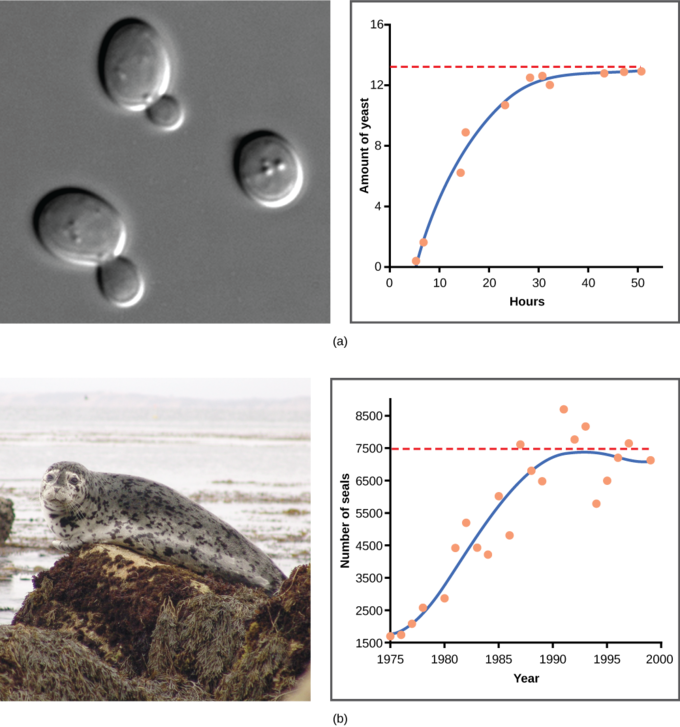
Yeast, a microscopic fungus used to make bread and alcoholic beverages, exhibits the classical S-shaped curve when grown in a test tube ( a). Its growth levels off as the population depletes the nutrients that are necessary for its growth. In the real world, however, there are variations to this idealized curve. Examples in wild populations include sheep and harbor seals ( b). In both examples, the population size exceeds the carrying capacity for short periods of time and then falls below the carrying capacity afterwards. This fluctuation in population size continues to occur as the population oscillates around its carrying capacity. Still, even with this oscillation, the logistic model is confirmed.

Figure \(\PageIndex{1}\): Logistic population growth: (a) Yeast grown in ideal conditions in a test tube show a classical S-shaped logistic growth curve, whereas (b) a natural population of seals shows real-world fluctuation.

Key Points

• The carrying capacity of a particular environment is the maximum population size that it can support.
• The carrying capacity acts as a moderating force in the growth rate by slowing it when resources become limited and stopping growth once it has been reached.
• As population size increases and resources become more limited, intraspecific competition occurs: individuals within a population who are more or less better adapted for the environment compete for survival.

Key Terms

• phenotype: the appearance of an organism based on a multifactorial combination of genetic traits and environmental factors, especially used in pedigrees
• carrying capacity: the number of individuals of a particular species that an environment can support; indicated by the letter “K”