A5. Experimental Analyses of Binding

It is often important to determine the Kd for a ML complex, since given that number and the concentrations of M and L in the system, we can predict if M is bound or not under physiological conditions. Again, this is important since whether M is bound or free will govern its activity. The trick in determining Kd is to determine ML and L at equilibrium. How can we differentiate free from bound ligand? The following techniques allow such a differentiation.

TECHNIQUES THAT REQUIRE SEPARATION OF BOUND FROM FREE LIGAND -

Care must be given to ensure that the equilibrium of \(M + L \rightleftharpoons ML\) is not shifted during the separation technique.

• gel filtration chromatography - Add M to a given concentration of L. Then elute the mixture on a gel filtration column, eluting with the free ligand at the same concentration. The ML complex will elute first and can be quantitated . If you measure the free ligand coming off the column, it will be constant after the ML elutes with the exception of a single dip near where the free L would elute if the column was eluted without free L in the buffer solution. This dip represents the amount of ligand bound by M.
• membrane filtration - Add M to radiolableled L, equilibrate, and then filter through a filter which binds M and ML. For instance, a nitrocellulose membrane binds proteins irreversibly. Determine the amount of radiolabeled L on the membrane which equals [ML].
• precipitation - Add a precipitating agent like ammonium sulfate, which precipitates proteins and hence both M and ML. Determine the amount of ML.

TECHNIQUES THAT DO NOT REQUIRE SEPARATION OF BOUND FROM FREE LIGAND

• concentrations ligand gives ML. Repeat at many different stoichiometry, which for a 1:1 ligande, determine the amount of bound or spectroscopic techniques. At equilibrium, determine free L by sampling the solution surrounding the bag. By mass balancradioisotopic whose concentration can be determined using ligand- Place M in a dialysis bag and dialyze against a solution containing a equilibirum dialysis.
• spectroscopy - Find a ligand whose absorbance or fluorescence spectra changes when bound to M. Alternatively, monitor a group on M whose absorbance or fluorescence spectra changes when bound to L.
• isothermal titration calorimetry (ITC)- In ITC, a high concentration solution of an analyte (ligand) is injected into a cell containing a solution of a binding partner (typically a macromolecule like a protein, nucleic acid, vesicle).

Figure: Isothermal Titration Calorimeter Cells

On binding, heat is either released (exothermic reaction) or adsorbed, causing a small temperature changes in the sample cell compared to the reference cells containing just a buffer solution. Sensitive thermocouples measure the temperature difference (DT1) between the sample and reference cells and apply a current to maintain the difference at a constant value. Multiple injections are made until the macromolecules is saturated with ligand. The enthalpy change is directly proportional to the amount of ligand bound at each injection so the observed signal attenuates with time. The actual enthalpy change observed must be corrected for the change in enthalpy on simple dilution of the ligand into buffer solution alone, determined in a separate experiment. The enthalpy changes observed after the macromolecule is saturated with ligand should be the same as the enthalpy of dilution of the ligand. A binding curve showing enthalpy change as a function of the molar ratio of ligand to binding partner (\(L_o/M_o\) if \(L_o \gg M_o\)) is then made and mathematically analyzed to determine Kd and the stoichiometry of binding.

Figure: Typical isothermal titration calorimetry data and analysis Reference: www.microcalorimetry.com/index.php?id=312

It should be clear in the example above, that the binding reaction is exothermic. But why is the graph of ΔH vs molar ratio of Lo/Mo sigmoidal (s-shaped) and not hyperbolic? One clue comes from the fact that the molar ratio of ligand (titrant) to macromolecule centers around 1 so, as explained above, when Lo is not >> Mo, the graph might not hyperbolic. The graphs below show a specific example of a Kd and ΔHo being calculated from the titration calorimetry data. They will shed light on why the graph of ΔH vs molar ratio of Lo/Mo is sigmoidal.

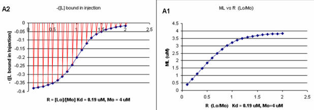
A specific example illustrates these ideas. Soluble versions of the HIV viral membrane protein, gp 120, 4 μM, was placed in the calorimetry cell, and a soluble form of its natural ligand, CD4, a membrane receptor protein from T helper cells, was placed a syringe and titrated into the cell (Myszka et al. 2000). Enthalpy changes/injection were determined and the data was transformed and fit to an equation which shows the ΔH "normalized to the number of moles of ligand (CH4) injected at each step". The line fit to the data in that panel is the best fit line assuming a 1:1 stoichiometry of CD4 (the "ligand") to gp 120 (the "macromolecule") and a Kd = 190 nM. Please note that the curve is sigmoidal, not hyperbolic.

Figure: Titration Calorimetry determination of Kd and DH for the interaction of gp120 and CD4

Note that the stoichiometry of binding (n), the KD, the ΔHo can be determined in a single experiment. From the value of ΔHo and KD, and the relationship

\[ΔGo = -RTlnKeq = RTlnKD = ΔHo - TΔSo\]

the ΔGo and ΔSo values can be calculated. No separation of bound from free is required. Enthalpy changes on binding were calculated to be -62 kcal/mol.

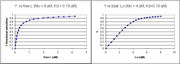
Using the standard binding equations (5, 7, and 10 above) to calculate free L and ML at a vary of Lo concentrations and R = Lo/Mo ratios, a series of plots can be derived. Two were shown earlier in this Chapter section to illustrate differences in Y vs L and Y vs Lo when Lo is not >> Mo. They are shown again below:

Figure: Y vs L and Y vs Lo when Lo is not >> Mo

Next a plot of ML vs R (= [Lo]/[Mo] (below, panel A1 right) was made. This curve appears hyperbolic but it has the same shape as the Y vs Lo graph above (right). However if the amount of ligand bound at each injection (calculated by subtracting [ML] for injection i+1 from [ML] for injection i) is plotted vs R (= [Lo]/[Mo]), a sigmoidal curve (below, panel A2, left) is seen, which resemble that best fit graph for the experimentally determine enthalpies above. The relative enthalpy change for each injection is shown in red. Note the graph in A2 actually shows the negative of the amount of ligand bound per injection, to make the graph look the that in the graph showing the actual titration calorimetry trace and fit above.

Figure: Binding Curves that Explain Sigmoidal Titration Calorimetry Data for gp120 and CD4

Surface Plasmon Resonance

A newer technique to measure binding is called surface plasmon resonance (SPR) using a sensor chip consisting of a 50 nm layer of gold on a glass surface. A carbohydrate matrix is then added to the gold surface. To the CHO matrix is attached through covalent chemistry a macromolecle which contains a binding site of a ligand. The binding site on the macromolecule must not be perturbed to any significant extent. A liquid containing the ligand is flowed over the binding surface.

The detection system consists of a light beam that passes through a prism on top of the glass layer. The light is totally reflected but another component of the wave called an evanescent wave, passes into the gold layer, where it can excite the Au electrons. If the correct wavelength and angle is chosen, a resonant wave of excited electrons (plasmon resonance) is produced at the gold surface, decreasing the total intensity of the reflected wave. The angle of the SPR is sensitive to the layers attached to the gold. Binding and dissociation of ligand is sufficient to change the SPR angle, as seen in the figure below.

• Fig: Surface Plasmon Resonance. (CC BY-SA 3.0; SariSabban)

animation: SPR evanaescent wave

This technique can distinguish fast and slow binding/dissociation of ligands (as reflected in on and off rates) and be used to determine Kd values (through measurement of the amount of ligand bond at a given total concentration of ligand or more indirectly through determination of both kon and koff.

Binding DB: a database of measured binding affinities, focusing chiefly on the interactions of protein considered to be drug-targets with small, drug-like molecules

PDBBind-CN: a comprehensive collection of the experimentally measured binding affinity data for all types of biomolecular complexes deposited in the Protein Data Bank (PDB).

Contributors and Attributions

• Prof. Henry Jakubowski (College of St. Benedict/St. John's University)