
4.1: Background
- Page ID
- 49688

In computer science, there is always a tendency to explore things that are somewhat similar to biological life. Computer scientists try to create programs which simulate real life features: growth, feeding, moving, reproduction and even evolution. These simulations help create robots, self-replicating systems and serve as steps toward artificial intelligence. From a biological point of view, such simulations demonstrate self-organization, or how organized life may emerge from a chaotic system of inorganic molecules. Modeling can support the hypothesis about the way that first cell likely formed billions years ago. And we can visualize how variation in design could give a creature an advantage over others in its population.
The most known simulation of this kind is a Conway’s Game of Life. This is not a game in a strict sense, it is more like programming. You will have a field of indefinite size, and a time (generations). The field is separated into dead cells (white) and live cells (black). Actually, the field is initially dead (white), and you will introduce black cells yourself. Every cell has 8 neighbors. Rules are simple:
-
A live cell with 2 or 3 (live) neighbors survives, but dies otherwise (easier to survive in groups).
-
A dead cell with exactly 3 (live) neighbors comes to life, and remains dead otherwise (reproduction).
As you understand, there may be infinite number of cell combinations. However, some of them are different. They behave, sometimes just like real cells. There is a classification:
-
Still lives. Creatures which do not change. Examples: block (left), boat (right) and others.
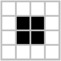.png?revision=1)
.png?revision=1)
Figure \(\PageIndex{1}\) -
Periodic / Quasi-periodic lives
-
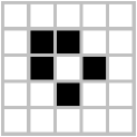
Oscillators. They change its shape cyclically. Examples: blinker (left), toad (right), 10 cell row, tumbler and others
.png?revision=1)
.png?revision=1)
Figure \(\PageIndex{2}\) -
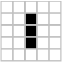
Spaceships (Translators). They are moving! Examples: glider (below), lightweight spaceship and others.
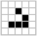
Figure \(\PageIndex{3}\)
-
-
Aperiodic lives
-
Transient lives. Sometimes, they just vanish. Sometimes, they live for a long time and only then stabilize. Examples: die hard (left), r pentomino (right), small exploder, exploder and others.
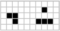.png?revision=1)
.png?revision=1)
Figure \(\PageIndex{4}\) -
Infinitely growing lives. They live forever and even produce offspring! These creatures are big and complicated. One of the smallest is Gosper glider gun (below).
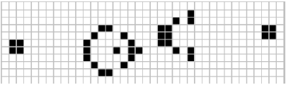
Figure \(\PageIndex{5}\)
-