7.1: Exponential Growth

At its simplest, changes in population size are determined by the relative balance of new members joining the population and current members leaving the population. For instance, new members may join the population through birth of new offspring or by immigration from other nearby populations of the species. Similarly, current members may leave the population through death or via emigration to other nearby populations. These processes can be represented mathematically:

\[\ce{Nt = N0 + B - D + I - E}\]

where N_t is the size of the population at a time in the future, which is the result of the current population size N₀, and the number of individual births (B), deaths (D), immigrants (I), and emigrants (E) that occur in that time interval. To estimate the population growth rate (the speed at which the population size changes through time), we can rewrite the previous equation as

\[\ce{∆N = B - D + I - E}\]

where ∆N represents the change in population size from time 0 to time t. If we consider a ‘closed’ population with no connection to other nearby populations, we can assume no change in population size from immigration or emigration, reducing our equation to

\[\ce{∆N = B - D}\]

Since the number of births and deaths that occur depend on the size of the population and the time length considered, it is important to convert numbers of births and deaths in the population into rates; the average number of births per individual per unit time (the per capita birth rate, b), and the average number of deaths per individual per unit time (the per capita death rate, d). These changes result in the following equation

\[\ce{∆N = (b-d) N0}\]

where N₀ is the population size at time 0. We can then summarize the per capita birth and death rates as the overall per capita growth rate r, which is the difference between the per capita birth and death rates. This change reduces the equation to

\[\ce{∆N = rN0}\]

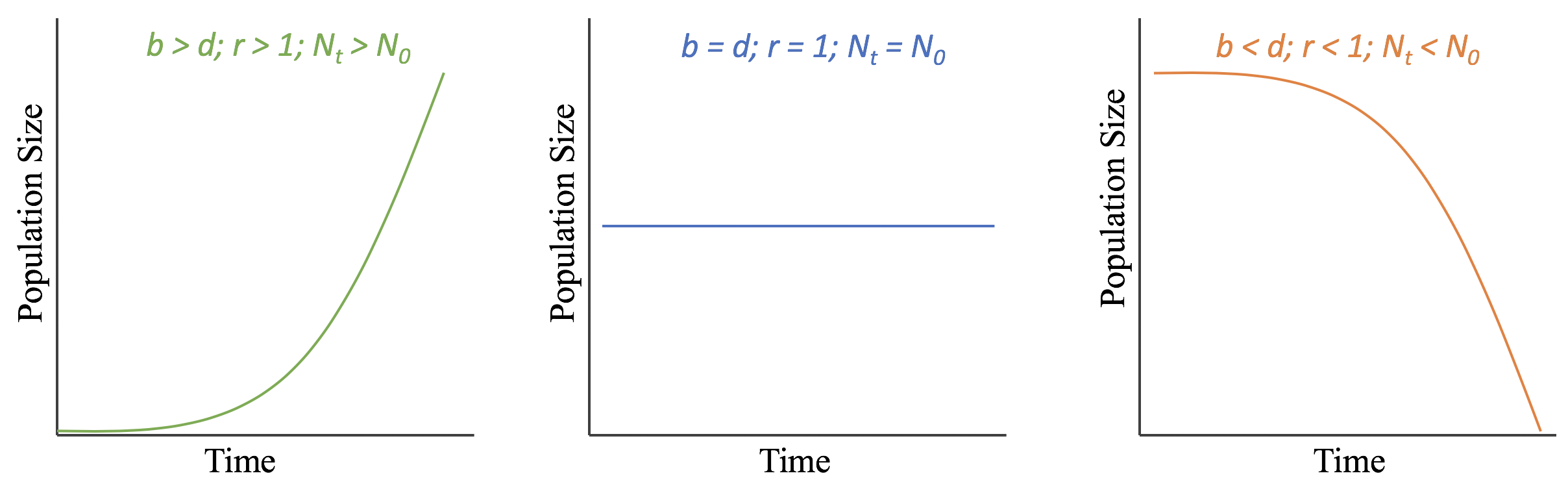
This equation represents the change in a population’s size through time given the balance between its birth and death rates. If birth rates are higher than death rates (b>d) then r >1 and the population size will increase through time (N_t>N₀). If birth rates are lower than death rates, (d>b) then r <1 and the population size will decrease through time (N_t<N₀). If birth and death rates are equal, (b=d) then r =1 and the population size will remain constant through time (N_t=N₀). Figure 7.1.1 illustrates these possible outcomes.

Figure \(\PageIndex{1}\): Illustrations of how the balance between birth rates (b) and death rates (d) affect population growth rates (r) and the population size through time. (Figures by L Gerhart-Barley.)

Using calculus, we can adjust the equation to represent very short, nearly instantaneous periods of time, which allow us to represent population growth as a curve instead of as discrete points along a line.

\[\ce{dN/dt = rN0}\]

Equation 7.1.6 allows us to predict the change in the size of a population across time, but it does not allow us to predict the actual population size at the end of that time period. In other words, we could estimate how many individuals might be added to or lost from the population, but not what the final number would be. Using calculus, we can integrate Equation 7.1.5 to an equation that does allow us to estimate future population size:

\[\ce{Nt = N0e^{rt}}\]

where e is a constant, the base of the natural log (e = 2.718) and t is the time interval between time 0 and time t. Knowing the current population size (N₀) and the per capita growth rate (r), we can then estimate the population size at future time t, which we call N_t.

This growth pattern is termed exponential growth because it results in the curvilinear growth trends illustrated in Fig 7.1.1, where large increases in the population occur as the population (N₀) increases. The pattern of increase also relates to the growth rate, r. When r is positive, higher r values will result in faster increases in population size than lower r values (Fig 7.1.2). When r is negative, lower (more negative) values of r lead to faster population decline. Consequently, the pattern of growth a population experiences is a result of both its current population size and its per capita growth rate.

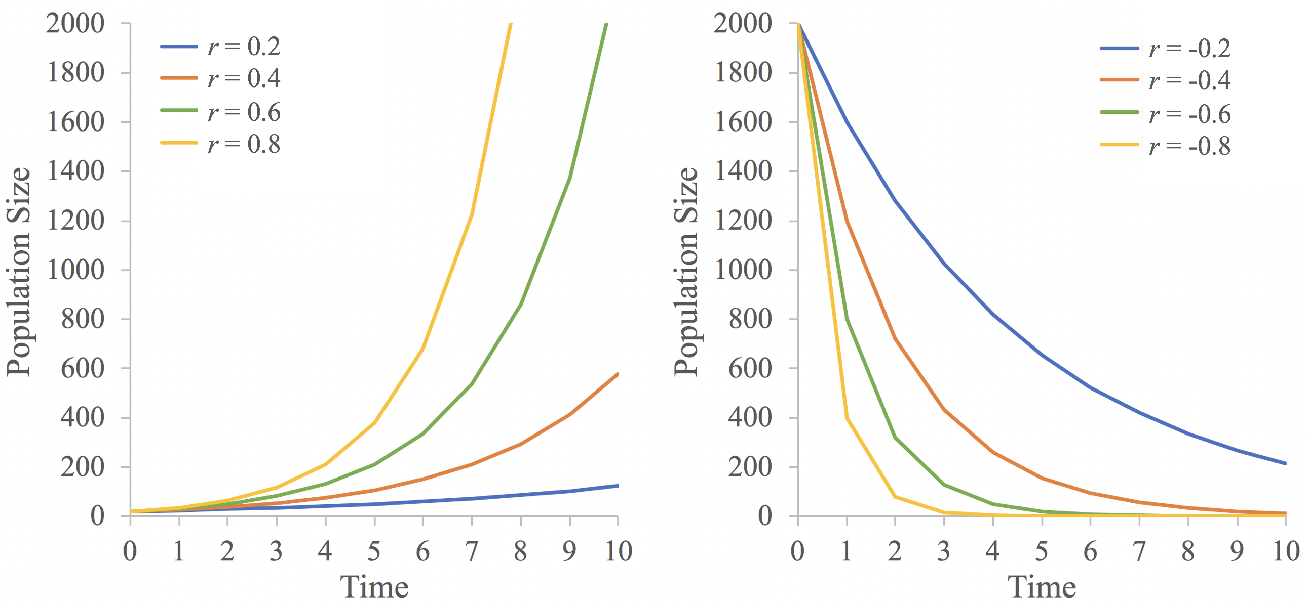
Figure \(\PageIndex{2}\): The influence of different values of \(r\) on population size through time. (Figure by L Gerhart-Barley)

Exponential Growth in Natural Populations

Some naturally-occurring populations exhibit exponential growth patterns. For example, pollen studies of sediment in Hockham Mere bog in Norfolk County, England spanning the last 10,000 show exponential growth in many tree species (Fig 7.1.3). These species expanded into Hockham Mere as glaciers retreated from the region, exposing new land area. While the details of the population growth patterns vary between the species, each shows the characteristic exponential pattern of initial slow growth when the population size is small, and more rapid growth as the population size increases.

Figure \(\PageIndex{3}\): Examples of exponential growth in populations of several tree genera surrounding Hockham Mere in Norfolk County, England following the retreat of glaciers from the area (Figure taken from Bennett et al 1983)

Exponential decline also occurs in populations. In some cases, this can be beneficial. For instance, viruses such as Hepatitis C and COVID-19, cannot survive indefinitely outside of a host. Consequently, viral populations infecting exposed surfaces experience exponential decline, reducing the risk of transmission of the viral infection over time. In other systems, however, such as the case of threatened and endangered species, exponential decline is of serious concern. For example, some loggerhead sea turtle populations in Japan and Australia have exhibited exponential decline in response to increasing sea surface temperatures caused by anthropogenic climate change (Fig 7.1.4).

Figure \(\PageIndex{4}\): Population sizes through time of four loggerhead sea turtle populations (a-d, right) and a map of the location of these populations (left). Figures from Chaloupka et al 2008.