Chemical Equilibrium—Part 2: Free Energy

Last updated
Save as PDF

Page ID: 9362

\( \newcommand{\vecs}[1]{\overset { \scriptstyle \rightharpoonup} {\mathbf{#1}} } \) \( \newcommand{\vecd}[1]{\overset{-\!-\!\rightharpoonup}{\vphantom{a}\smash {#1}}} \)\(\newcommand{\id}{\mathrm{id}}\) \( \newcommand{\Span}{\mathrm{span}}\) \( \newcommand{\kernel}{\mathrm{null}\,}\) \( \newcommand{\range}{\mathrm{range}\,}\) \( \newcommand{\RealPart}{\mathrm{Re}}\) \( \newcommand{\ImaginaryPart}{\mathrm{Im}}\) \( \newcommand{\Argument}{\mathrm{Arg}}\) \( \newcommand{\norm}[1]{\| #1 \|}\) \( \newcommand{\inner}[2]{\langle #1, #2 \rangle}\) \( \newcommand{\Span}{\mathrm{span}}\) \(\newcommand{\id}{\mathrm{id}}\) \( \newcommand{\Span}{\mathrm{span}}\) \( \newcommand{\kernel}{\mathrm{null}\,}\) \( \newcommand{\range}{\mathrm{range}\,}\) \( \newcommand{\RealPart}{\mathrm{Re}}\) \( \newcommand{\ImaginaryPart}{\mathrm{Im}}\) \( \newcommand{\Argument}{\mathrm{Arg}}\) \( \newcommand{\norm}[1]{\| #1 \|}\) \( \newcommand{\inner}[2]{\langle #1, #2 \rangle}\) \( \newcommand{\Span}{\mathrm{span}}\)\(\newcommand{\AA}{\unicode[.8,0]{x212B}}\)

In a previous section, we began a description of chemical equilibrium in the context of forward and reverse rates. Three key ideas were presented:

At equilibrium, the concentrations of reactants and products in a reversible reaction are not changing in time.
A reversible reaction at equilibrium is not static—reactants and products continue to interconvert at equilibrium, but the rates of the forward and reverse reactions are the same.
We were NOT going to fall into a common student trap of assuming that chemical equilibrium means that the concentrations of reactants and products are equal at equilibrium.

Here we extend our discussion and put the concept of equilibrium into the context of free energy, also reinforcing the Energy Story exercise of considering the "Before/Start" and "After/End" states of a reaction (including the inherent passage of time).

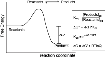
Figure 1. Reaction coordinate diagram for a generic exergonic reversible reaction. Equations relating free energy and the equilibrium constant: R = 8.314 J mol^-1 K^-1 or 0.008314 kJ mol^-1 K^-1; T is temperature in Kelvin.

Attribution: Marc T. Facciotti (original work)

The figure above shows a commonly cited relationship between ∆G° and K_eq: ∆G° = -RTlnK_eq. Here, G° indicates the free energy under standard conditions (e.g., 1 atmosphere of pressure, 298K). In the context of an Energy Story, this equation describes the change in free energy of a reaction whose starting condition is out of equilibrium; specifically, all matter at the "start" is in the form of reactants, and the "end" of the reaction is the equilibrium state. Implicit is the idea that the reaction can theoretically proceed to infinite time so that no matter the shape of its energy surface, it can reach equilibrium. One can also consider a reaction where the "starting" state is somewhere between the starting state above and equilibrium and perhaps where the reaction is not at equilibrium. In this case, one can examine the ∆G (not standard conditions) between the "intermediate" starting state and equilibrium by considering the equation ∆G = ∆G° + RTlnQ, where Q is called the reaction quotient. From the standpoint of BIS2A, we will use a simple (a bit incomplete but functional) definition for Q = [Products]_st/[Reactants]_stat a defined non-equilibrium "starting" condition st. The equation ∆G = ∆G° + RTlnQ can therefore be read as the free energy of the transformation being equal to the free energy associated with the free energy difference for ideal standard condition plus the contribution of free energy that represents the deviation away from the "ideal" starting state represented by the actual starting state and conditions. In both cases, the "final" condition is still equilibrium; we are just changing starting points. One can extend this idea and calculate the free energy difference between two non-equilibrium states, provided they are properly defined, but that's for your chemistry instructor to bother you with. The key point here is that there is a way to both conceive of and compute free energy changes between specifically defined states, not just the standard initial state and equilibrium as the end state.

This takes us to the core summary point. In many biology books, the discussion of equilibrium includes not only the discussion of forward and reverse reaction rates, but also a statement that ∆G = 0 at equilibrium. This often confuses some students because they are also taught that a nonzero ∆G can be associated with a reaction going to equilibrium. We do this each time we report the ∆G of a reaction or examine a reaction coordinate diagram. So, students tend to memorize the "∆G=0 at equilibrium" statement without appreciating where it comes from. The key to closing the apparent disconnect for many is to appreciate that the interpretation of the sometimes seemingly contradictory statements depend a lot on the definition of the starting and ending states used to calculate ∆G. In the case of reporting ∆G for a reaction, the starting state was described in the paragraphs above (in one of two ways—either standard conditions or non-standard, out-of-equilbrium state), and the ending state is some time later, once the reaction has reached equilibrium. Since the starting and ending states are different, ∆G can be nonzero, positive, or negative. By contrast, the statement that concludes "∆G=0 at equilibrium" is considering a different starting state. In this case, the starting state is the system already at equilibrium. The ending state is considered to be sometime later, but still at equilibrium. Since the starting and ending states are ostensibly the same, ∆G = 0.