1.14: Deviations from Mendelian Genetics- Linkage (Part 1)

Learning Objectives

At the completion of this lesson, you will be able to:

1. Contrast the inheritance of traits that are controlled by independent genes, linked genes and pleiotropic genes.
2. Demonstrate the physical basis of linkage by drawing the key events in meiosis.
3. Calculate map distances from 2-point test cross and F2 data.
4. Assemble linkage maps from map distance information.

Maize Genetics

Maize (Zea mays, corn) is not only a commercially important crop; it has also been a valuable organism used in basic genetic studies to understand genetic principles. Geneticists such as Dr. John Osterman, in the School of Biological Sciences at the University of Nebraska, use corn in basic genetic studies. Let’s examine one experiment.

Many seed traits in corn have been studied by geneticists. Color in the outside (aleurone) or inside (endosperm) of the seed can be important for end uses such as what color of corn chips you prefer. Starch development traits in the kernel influence what the corn seed can be used for (popcorn, sweet corn, waxy corn).

A line of corn that was true breeding for a red kernel color was crossed to a true breeding line with shrunken kernels but no red color (white or yellow). Even though the two parents differed by two traits, kernel color and kernel shape, the F₁ offspring produced from the cross were all red with plump or normal kernels.

Parents: Red, plump x white, shrunken

F₁ offspring: All red, plump

Which phenotypes would you say are dominant based upon this single result? Going a step further, what is your hypothesis for the genotypes of the parents and F₁?

The next year these red plump seeds were planted in the crossing nursery near the white shrunken line. Dr. Osterman made a backcross or testcross between the F₁ progeny and white, shrunken plants.

Thinking back on the genetics principles we have covered so far in this course, what phenotypes would you expect to observe in the testcross progeny?

If we use the principle of independent assortment and the information we already have, we would predict that there should be four types of seeds in testcross progeny.

Figure 1. Seed trait inheritance in test cross progeny assuming independent assortment. Image by Donald Lee.

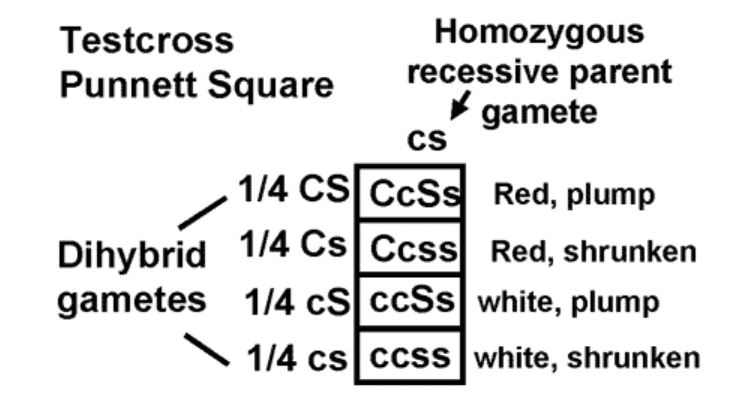
We should get both parental combinations of red, plump and white, shrunken. We should also get two new combinations; red, shrunken and white, plump. Furthermore, the principle of independent assortment predicts the four combinations should be in a 1:1:1:1 ratio. (Make sure you understand why!)

Figure 2. Testcross progeny showing red, plump and white, shrunken phenotype. Image by Donald Lee.

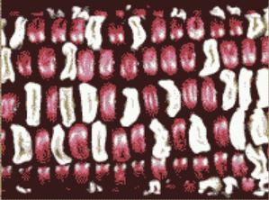
What did Dr. Osterman actually observe? When he harvested the ear from the first plant, peeled back the husks, and examined the kernels, all he saw were red, plump and white, shrunken seeds. Only the parental combination of traits was found among the several hundred seeds on that ear!

Half the seeds had the dominant red and plump combination while the other half had the recessive traits. While this result does not fit what we expect based on the idea of independent traits, Dr. Osterman was not surprised. Obviously, another genetic hypothesis can explain this result. Let’s examine two alternative explanations.

Pleiotropy

Sometimes a single gene pair will control more than one trait. For example, barley that has good malting characteristics for brewing also tends to sprout prior to harvest. High sucrose lines of soybean have a sweeter flavor in soymilk and cause less gas production in the consumer compared to lines with normal sucrose levels. Perhaps a seed color gene in corn also controls whether the kernel is plump or shrunken. White kernels would always be shrunken, red would always be plump. When genes control more than one trait, these traits will always be inherited together. This explanation is consistent with what Dr. Osterman observed on the seeds of the testcross ear.

Linkage

The second explanation involves two genes but looks closely at their chromosome locations. Cytogeneticists have observed ten pairs of chromosomes in the somatic cells of corn. Corn has countless traits controlled by tens of thousands of genes. Since genes are on chromosomes, it makes logical sense that each chromosome is made of thousands of genes. When genes are on the same chromosome they will travel together as the chromosome is passed on to the gametes (Figure 3). If the gene for red vs. white kernel color is on the same corn chromosome as the gene for plump vs. shrunken, those genes will travel together during gamete formation. This could also explain why the red and plump gene alleles are inherited together. The same would be true of the white and shrunken alleles on the homologous chromosome in the F₁. Therefore, we could explain the result by the hypothesis of linkage; a separate gene pair controls each trait but these genes are located near each other on the same chromosome.

Figure 3. Genes located on the same chromosome are genetically linked. Genetic linkage analysis can be used to determine the order of genes on chromosomes. Closely linked genes are not segregating independently, like genes located on different chromosomes. Linked genes can be used as genetic markers, which have become an important tool in plant breeding. Image by Walter Suza.

More Data

Two genetic hypotheses can explain the testcross data. How can we determine which hypothesis is correct? Like all good geneticists, Dr. Osterman made an effort to generate large numbers of offspring in his studies. He had made several test crosses that summer and each cross generated ears with several hundred seeds. Upon careful examination of the seeds on all the ears, Dr. Osterman did observe a few red shrunken and white plump kernels. The new combinations were rare but their appearance in the testcross progeny allows us to eliminate one of the genetic hypotheses. Which hypothesis can be ruled out?

Linked Genes Tend to Stay Together

Because the red trait and plump trait are not always found together, one gene cannot be responsible for both traits, the occurrence of the recombinant red, shrunken and white, plump testcross offspring eliminates this as a reasonable hypothesis. Can we still use linkage as an explanation though? Yes, if we think through chromosome behavior during meiosis, we can see why genes on the chromosome tend to stay together but will not always be passed on together. Let’s think about meiosis and crossing over to understand these results.

Crossing Over

Figure 4. Crossover not between C,c and S,s. Only CS and cs. Parental gametes are made. Image by Marjorie Hanneman.

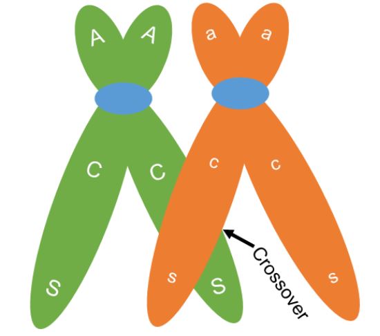
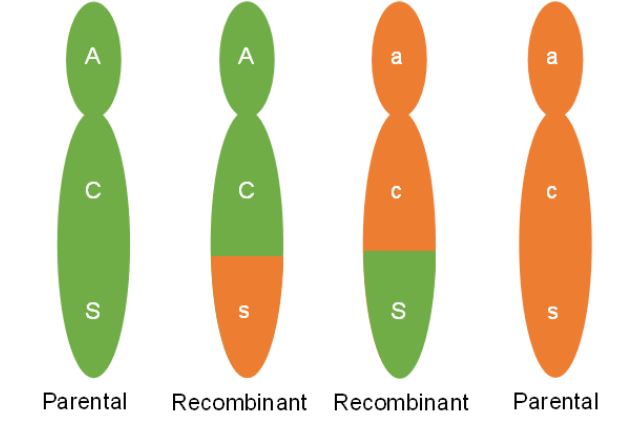
One of the key differences between meiosis and mitosis is the synapsis of homologous chromosomes during prophase I of meiosis. Synapsis is the process in which homologous chromosomes carefully pair. The pairing allows for an orderly first division to send one chromosome from each pair to separate cells. The close association of the homologous chromosomes also allows for crossing over between non-sister chromatids (Figure 4). During this process sections of the chromosomes break off and are exchanged between non-sister chromatids. When non-sister chromatids crossover, chromatids can be made that have a new combination of genes compared to the original combination on the chromosome. The original combination was inherited from the organism’s parents and is called the parental combination of genes. The new combination made is called the recombinant combination. In figure 4, a crossover occurs but the original or parental combination of CS (red and plump) and cs (white and shrunken) will stay together. Crossing over can cause new gene combinations to occur on a chromosome if the crossover occurs between the linked genes.

Figure 5. Crossover between the C,c and S,s gives Cs and cS recombinant plus CS and cs parental. Image by Marjorie Hanneman.

When a crossover occurs between genes, chromatids with both the parental combination and chromatids with a new combination will be made. We can see this in figure 5. Two of the chromatids are not involved in the crossing over. These chromatids will maintain the parental combination and when meiosis is complete, the two gametes made that have these chromosomes will be called parental gametes. The gametes made that have the other two chromosomes, those that went through crossing over and have the new gene combination, are called recombinant gametes (Figure 6).

Figure 6. Parental and recombinant gametes from crossovers between C,c and S,s. Image by Marjorie Hanneman.

When crossing over occurs between two non-sister chromatids, cells will make equal numbers of recombinant and parental gametes. In looking back at Dr. Osterman’s data though the number of plants that would have inherited recombinant type gametes was far below 50%. Why are parental combinations of linked genes made more frequently than new combinations? Understanding this requires us to imagine many cells going through gamete formation.

Making Lots of Gametes

Sexually reproducing organisms tend to make a large number of gametes to ensure reproductive success. Therefore, we need to think about crossing over events happening in many cells. Geneticists do not understand all the details of crossing over but in general, crossing over is a random process that occurs during prophase I. We also know that the occurrence of one crossover along a chromosome can reduce the chance of a second crossing over. As you look at figure 5, you can see that crossing over could occur at any point between where the C,c genes (the C,c locus) and the S,s locus reside on the chromosome causing recombinant gamete formation. If a crossover does not occur between the C,c and S,s loci (plural for locus), then only the parental gamete combination of CS and cs will be made. Considering the size of the chromosome and the relative positions of the C,c and S,s loci; how often would cells have crossovers occur between the genes compared to somewhere else along the chromosome? If crossing over is random, we would not expect a cross over to occur in very many cells between the C,c and S,s loci. Genes that are on the same chromosome tend to stay together at a rate that is proportional to how far apart they are on the chromosome. Since the C,c and S,s loci are close to each other, crossovers are rare. The ‘C’ gene tends to stay with the ‘S’ gene as it is passed from the red, plump line to the F1 and then to the testcross generation. The same is true of the ‘c’ and ‘s’ parental combination.

How does this discussion of crossing over help us understand what we see from our test cross result? The parental combinations of red, plump, and white shrunken were almost always made. The new combinations of red, shrunken and white, plump were rarely observed. It would take a recombinant gamete to make one of these rare combinations. While we never see the genes in the gametes or directly observe the genes on the chromosomes, the outcome suggests that these loci are linked close together on the chromosome. Making the connection between the results of crossing studies such as these has allowed geneticists to map genes or determine their relative positions on a chromosome. Let’s go through a mapping study to see how it is done.

Two-Point Testcross Mapping

The results of a testcross study different from Dr. Osterman’s is given below

• Red, Shrunken CCss X White, Plump ccSS
• F₁: all Red, Plump (CcSs)
• F₁ (CcSs) crossed with White Shrunken (ccss)

Table 1. Testcross progeny data

Phenotypes

# of progeny

Red, plump

120

Red, shrunken

3420

White, plump

3334

White, shrunken

126

Total

7000

Obviously, the geneticist who did this experiment made a lot of test crosses to generate these numbers. How can we use the numbers to map these genes? With this information we can answer one question. ‘What is the distance between the C,c and S,s loci?’ We cannot get out a fancy microscopic ruler and physically measure the distance on the corn chromosome. With this information all we can do is estimate the map unit distance. Map units are a measure of the tendency for crossovers to occur between two loci. Because genes that are farther apart will have a higher likelihood of crossovers, the higher the crossover frequency, the farther apart the genes are on the chromosome. Let’s apply this idea to our test cross data.

Test cross data allows us to indirectly measure the frequency of gametes made by an individual. All of the testcross progeny inherited a gamete with the recessive ‘c‘ and ‘s‘ alleles from the white, shrunken parent. Therefore, the alleles that the F₁, dihybrid parent has passed on determine the traits in the seed (Table 1). We need to be able to measure how often crossovers occurred between the C,c and S,s loci when these dihybrids made gametes. From the data we have the following:

• Gametes that were passed to the F₁ from the parent lines were Cs and cS.
• Gametes made from crossing over in the F₁ (recombinant gametes) were CS and cs.
• Gametes with the original parent combination (parental gametes) were Cs and cS.

Therefore, the frequency of recombinant gametes was 246 (120 + 126) divided by the total gametes we have information on (7000) or 246/7000 = 3.5%

Map unit distance between the C,c and S,s loci = 3.5 Map units.

One map unit is equal to 1% recombinant gametes. Again, this is not a physical measurement. It is a relative measure of how often crossovers occurred between these loci. How reliable is this measurement? Let’s look at another data set (Table 2).

• Red, plump CCSS X White, shrunken ccss
• F₁: all Red, Plump (CcSs or CS / cs)
• F₁ (CS / cs) crossed with White Shrunken (ccss)

Table 2. Testcross progeny data from another data set

Phenotypes

# of Progeny

Red, plump

192

Red, shrunken

5

White, plump

3

White, shrunken

200

Total

400

Recombinant gamete frequency: 5 + 3 / 400 = 2%; 2 map units from C,c to S,s

Based on this result is the map unit distance measurement reliable? Yes, it is, to a certain degree. It is important to recognize the differences between the two test cross experiments.

Cis Versus Trans

Figure 7. Dihybrid in Cis. Image by Marjorie Hanneman.

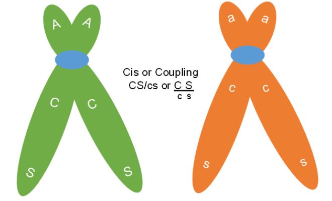
The first difference to note is that the parental gametes are not always the same allele combinations, but they are always the most frequently produced gametes. In the smaller experiment above, the parents had either both dominant or both recessive traits together. Therefore, the F₁ parent was making Cs and cS recombinant gametes. This dihybrid parent was in cis or coupling phase with respect to these genes (Figure 7).

Figure 8. Dihybrid in Trans. Image by Marjorie Hanneman.

In the larger experiment with 7000 testcross progeny the dihybrid F₁ was in trans or repulsion phase for the C,c and S,s genes. In this case the Cs and cS are the parental gametes (Figure 8). Therefore, when genes are linked, they can be arranged in two ways in a dihybrid. This means that a CcSs plant can have its genotype in the cis arrangement with both dominant genes on one chromosome and both recessives on the other (written CS / cs) or can also be in trans (Cs / cS).

Map Distance Measurement

The first experiment gave us 3.5 map units and the latter gave 2 map units.

Why do our two experiments give us two different map unit distances? In both cases, we can see that the parental gene combinations have a strong tendency to stay together. Because the experiments were done with different population sizes, with different plants, and the difference in our map unit estimates is small, the difference could be attributed to chance. Environment may also influence the rate of crossing over to some degree. For practical purposes this gene mapping information is reliable enough to tell us that these two genes reside close to each other on the same chromosome. Once we have information on distances between other genes, we can improve our map.

Mapping Another Seed Trait Gene Pair

A third seed trait in corn is normal vs. waxy starch. Waxy starch has a different chemistry than normal starch and can be scored by staining with iodine. This gene is commercially important because some waxy corn is produced for specialty markets. Let’s look at the following test cross data (Table 3):

Parent: Red, Normal (CCWW) X White, waxy (ccww)

F₁: Red, Normal (CcWw) X White, Waxy (ccww)

Table 3. Testcross data for another seed trait

Phenotypes

# of testcross progeny

Red, normal

2781

Red, waxy

759

White, normal

749

White, waxy:

2711

Total

7000

• Parental gametes made by the F₁: CW and cw
• Recombinant gametes made by the F₁: Cw and cW = 759 + 749 = 1508
• Map unit distance between the C,c and the W,w loci: 1508/7000 = 21.5 Map Units

It is clear from the testcross data (Table 3) that the genes at the C,c and W,w loci do not have as great a tendency to be inherited together compared to the genes at the C,c and S,s loci. This would be because the loci are farther apart, and our 21.5 map units is an indicator of the relative distance.

Figure 9. Two possible linkage maps from two-point data. Image by Donald Lee.

From the two distances calculated, how far apart are the W,w and S,s loci? Here is where we can try to use map unit distances to do gene mapping the same way we use miles to do road mapping. We can pencil our two possible maps (Figure 9).

In one map the C,c locus is in between the W,w and S,s loci. Using the 21.5 plus 3.5 map units we have calculated, the best estimate will be that 25 map units separate the W,w and S,s loci. The other map that fits our data is having the S,s locus in the middle with the W,w and S,s loci 18 map units apart (21.5 – 3.5). If the genes occupy a fixed position on the chromosome, only one map will be correct. How can we determine which is the correct map?

The Third Map Distance

A third map distance needs to be estimated in order to determine the linkage map of these three loci. We need to make a cross that gives us the opportunity to measure crossing over frequency between the S,s and W,w loci. One such cross is shown below.

• Parent: ssWW (shrunken, normal) X SSww (plump, waxy)
• F₁: sW / Sw X sW / Sw

Test cross offspring:

Plump, normal:

630

Plump, waxy:

2824

Shrunken, normal:

2900

Shrunken, waxy:

646

Total:

7000

• Recombinant gametes: 646 + 630 = 1276
• Map distance S,s to W,w: 1276/7000 = 18/2 map units

Based on the third map distance our best map for all three loci is the second alternative (Figure 9). To map all three loci using this two-point test cross data, the geneticist needed to generate three different crosses. This is how gene maps in organisms such as corn have been generated. As new genes controlling traits are discovered, crosses can be made to test if these genes are independent or linked to other genes. Once linkage is determined, additional crosses can be analyzed to position the gene on the linkage map.

Map Distances from F₂ Data

In our last test cross, the F₁ dihybrid sW / Sw was crossed to a sw/sw, shrunken waxy plant. If the shrunken waxy line was not available, the geneticist could still obtain information to determine map distance by selfing the F₁ to produce F₂ offspring. Here is the procedure.

Results of Selfing the sW/Sw F₁:

F2 Offspring

Number

Plump, normal

254

Plump, waxy

122

Shrunken, normal

120

Shrunken, waxy

4

Total F2s:

500

Step one: Focus on the double recessive (sw/sw).

How do we obtain recombinant gamete frequencies from this F₂ phenotype information? The first thing to remember is that this is a self-cross rather than a testcross and an additional Punnett square is needed to depict how gametes produced these F₂ (Figure 10). From the Punnett square we can see that four kinds of gametes are made in both the male and female in this cross. Therefore, the plump, normal seeds can be made nine different ways in our diagram and will consist of five different genotypes (SW/SW, SW/sW, sW/SW, sW/Sw and SW/sw). We cannot tell by observing the seed phenotype though, which of the genotypes it has. The plump, waxy and shrunken, normal F₂ seeds will each consist of two different genotypes. The only F₂ phenotypes that consist of a single genotype are the shrunken, waxy. They are all ssww (sw/sw). By focusing on how this phenotype was produced in the F₂, we can estimate the frequency of recombinant gametes made by the selfed parent.

Figure 10. Mapping from F₂ data. Focus with the method described is on the double recessive, ssww or sw/sw, F₂. Image by Donald Lee.

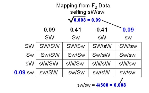
Step two: Go from phenotype frequency to gamete frequency.

Look at the Punnett square and think about how the shrunken waxy seeds were made. First, a sw gamete in the male part of the plant and a sw gamete in the female needed to be made. The parent had the genotype sW/Sw that means that these would be recombinant gametes in both the male and female. Once these gametes were made, they needed to come together at random during pollination to produce the seed. Mathematically, we can say that the frequency of the shrunken, waxy seeds is the frequency of the sw gamete made in the male times the frequency of the sw gamete made in the female. If we assume that crossovers occur in the pollen forming cells at the same frequency as the egg forming cells, then the frequency of the shrunken waxy seeds is the square of the frequency of sw. Make sure this last paragraph makes sense to you by walking through figure 10.

Step three: Take the square root.

Now we can use our seed phenotype frequency to estimate gamete frequency in the selfed parent. Four of the 500 seeds produced were shrunken waxy. That would give our square in the lower right a frequency of 0.008 (4/500). This frequency should be the sw gamete frequency squared (sw2). If we want to know the frequency of sw, we can take the square root of 0.008 and get about 0.09. Now we have the frequency of one gamete estimated. This would be the same for both the male and female gametes, where 9% of all gametes produced by the sW/Sw parent will be sw. As it turns out, we can calculate the frequency of the other three gametes from this information if we just think about how the gametes were made in meiosis.

Step four: Double the frequency, decide if parental or recombinant.

In our continuing example the sw gamete was made when a crossover occurred in the sW/Sw parent. Crossovers are a reciprocal exchange between non-sister chromatids so every time a sw gamete was made, a SW gamete was also made. Therefore, if the sw frequency is 0.09 then the SW frequency is also 0.09. These are our recombinant gametes, so the frequency of recombinant gametes is 2 X 0.09 or 0.18. We can tell from this frequency that these are the recombinant gametes, they are less frequently made than the parental gametes. The parental gametes would total 82% of the gametes, each parental gamete making up half (41%) of that total. Thus, 18 map units between the S,s and W,w loci is our map distance estimate from the data. Because we use only a subset of the information in this procedure (only the double recessive numbers) this estimate is more subject to chance than the test cross data. We can use more complex math to estimate gamete frequencies from all the F₂ data but this square root method is a quick way to detect linkage and estimate map distance. In cases where geneticists cannot perform a testcross working with F₂ data is a necessary part of gene mapping. Can you think of some instances where this would be true?