5.3: Modeling the evolution of correlated characters

Last updated
Save as PDF

Page ID: 21602

$ \newcommand{\vecs}[1]{\overset { \scriptstyle \rightharpoonup} {\mathbf{#1}} } $ $ \newcommand{\vecd}[1]{\overset{-\!-\!\rightharpoonup}{\vphantom{a}\smash {#1}}} $$\newcommand{\id}{\mathrm{id}}$ $ \newcommand{\Span}{\mathrm{span}}$ $ \newcommand{\kernel}{\mathrm{null}\,}$ $ \newcommand{\range}{\mathrm{range}\,}$ $ \newcommand{\RealPart}{\mathrm{Re}}$ $ \newcommand{\ImaginaryPart}{\mathrm{Im}}$ $ \newcommand{\Argument}{\mathrm{Arg}}$ $ \newcommand{\norm}[1]{\| #1 \|}$ $ \newcommand{\inner}[2]{\langle #1, #2 \rangle}$ $ \newcommand{\Span}{\mathrm{span}}$ $\newcommand{\id}{\mathrm{id}}$ $ \newcommand{\Span}{\mathrm{span}}$ $ \newcommand{\kernel}{\mathrm{null}\,}$ $ \newcommand{\range}{\mathrm{range}\,}$ $ \newcommand{\RealPart}{\mathrm{Re}}$ $ \newcommand{\ImaginaryPart}{\mathrm{Im}}$ $ \newcommand{\Argument}{\mathrm{Arg}}$ $ \newcommand{\norm}[1]{\| #1 \|}$ $ \newcommand{\inner}[2]{\langle #1, #2 \rangle}$ $ \newcommand{\Span}{\mathrm{span}}$$\newcommand{\AA}{\unicode[.8,0]{x212B}}$

We can model the evolution of multiple (potentially correlated) continuous characters using a multivariate Brownian motion model. This model is similar to univariate Brownian motion (see chapter 3), but can model the evolution of many characters at the same time. As with univariate Brownian motion, trait values change randomly in both direction and distance over any time interval. Here, though, these changes are drawn from multivariate normal distributions^². Multivariate Brownian motion can encompass the situation where each character evolves independently of one another, but can also describe situations where characters evolve in a correlated way.

We can describe multivariate Brownian motion with a set of parameters that are described by a, a vector of phylogenetic means for a set of r characters:

(eq. 5.1)

\[ \mathbf{a} = \begin{bmatrix} \bar{z}_1 (0) & \bar{z}_2 (0) & \dots & \bar{z}_r (0)\\ \end{bmatrix} \]

This vector represents the starting point in r-dimensional space for our random walk. In the context of comparative methods, this is the character measurements for the lineage at the root of the tree. Additionally, we have an evolutionary rate matrix R:

(eq. 5.2)

\[ \mathbf{R} = \begin{bmatrix} \sigma_1^2 & \sigma_{21} & \dots & \sigma_{n1}\\ \sigma_{21} & \sigma_2^2 & \dots & \vdots\\ \vdots & \vdots & \ddots & \vdots\\ \sigma_{1n} & \dots & \dots & \sigma_{rn}^2\\ \end{bmatrix}\]

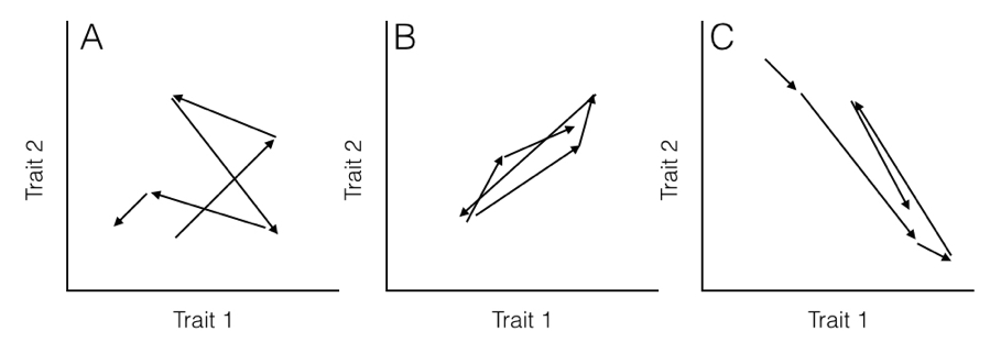
Here, the rate parameter for each axis (σ_i²) is along the matrix diagonal. Off-diagonal elements represent evolutionary covariances between pairs of axes (note that σ_ij = σ_ji). It is worth noting that each individual character evolves under a Brownian motion process. Covariances among characters, though, potentially make this model distinct from one where each character evolves independently of all the others (Figure 5.2).

Figure 5.2. Hypothetical pathways of evolution (arrows) for (A) two uncorrelated traits, (B) two traits evolving with a positive covariance, and (C) two traits evolving with a negative covariance. Note that in (B), when trait 1 gets larger trait 2 also gets larger, but in (C) positive changes in trait 1 are paired with negative changes in trait 2. Image by the author, can be reused under a CC-BY-4.0 license.

When you have data for multiple continuous characters across many species along with a phylogenetic tree, you can fit a multivariate Brownian motion model to the data, as discussed in Chapter 3.

To calculate the likelihood, we can use the fact that, under our multivariate Brownian motion model, the joint distribution of all traits across all species has a multivariate normal distribution. Following Chapter 3, we find the variance-covariance matrix that describes that model by combining the two matrices R and C into a single large matrix using the Kroeneker product:

(eq. 5.3)

V = R ⊗ C

This matrix V is nr × nr. We can then substitute V for C in equation (4.5) to calculate the likelihood:

(eq. 5.4)

\[ L(\mathbf{x}_{nr} | \mathbf{a}, \mathbf{R}, \mathbf{C}) = \frac {e^{-1/2 (\mathbf{x}_{nr}- \mathbf{D} \cdot \mathbf{a})^\intercal (\mathbf{V})^{-1} (\mathbf{x}_nr-\mathbf{D} \cdot \mathbf{a})}} {\sqrt{(2 \pi)^{nm} det(\mathbf{V})}} \]

Here D is an nr × r design matrix where each element D_ij is 1 if (j − 1)⋅n < i ≤ j ⋅ n and 0 otherwise. x_nr is a single vector with all trait values for all species, listed so that the first n elements in the vector are trait 1, the next n are for trait 2, and so on:

(eq. 5.5)

\[ \mathbf{x}_{nr} = \begin{bmatrix} x_{11} & x_{12} & \dots & x_{1n} & x_{21} & \dots & x_{nr}\\ \end{bmatrix} \]

We can find the value of the likelihood at its maximum by calculating L(x_nr|a, R, C) using eq. 5.4 and an optimization routine to find the MLE.

Alternatively, one can calculate this MLE solution directly. Equations for estimating $\hat{\mathbf{a}}$ (the estimated vector of phylogenetic means for all characters) and $\hat{\mathbf{R}}$ (the estimated evolutionary rate matrix) are (Revell and Harmon 2008, Hohenlohe and Arnold (2008)):

(eq. 5.6)

\[ \hat{\mathbf{a}} = [(\mathbf{1}^\intercal \mathbf{C}^{-1} \mathbf{1})^{-1}(\mathbf{1}^\intercal \mathbf{C}^{-1} \mathbf{X})]^\intercal \]

(eq. 5.7)

\[ \hat{\mathbf{R}} = \frac{(\mathbf{X} - \mathbf{1} \mathbf{\hat{a}})^\intercal \mathbf{C}^{-1} (\mathbf{X} - \mathbf{1} \mathbf{\hat{a}})}{n} \]

Note here that we use X to denote the n (species) × r (traits) matrix of all traits across all species. Note the similarity between these multivariate equations (5.6 and 5.7) and their univariate equivalents (equations 4.6 and 4.7).