4.4: Bayesian approach to evolutionary rates

Last updated
Save as PDF

Page ID: 21595

$ \newcommand{\vecs}[1]{\overset { \scriptstyle \rightharpoonup} {\mathbf{#1}} } $ $ \newcommand{\vecd}[1]{\overset{-\!-\!\rightharpoonup}{\vphantom{a}\smash {#1}}} $$\newcommand{\id}{\mathrm{id}}$ $ \newcommand{\Span}{\mathrm{span}}$ $ \newcommand{\kernel}{\mathrm{null}\,}$ $ \newcommand{\range}{\mathrm{range}\,}$ $ \newcommand{\RealPart}{\mathrm{Re}}$ $ \newcommand{\ImaginaryPart}{\mathrm{Im}}$ $ \newcommand{\Argument}{\mathrm{Arg}}$ $ \newcommand{\norm}[1]{\| #1 \|}$ $ \newcommand{\inner}[2]{\langle #1, #2 \rangle}$ $ \newcommand{\Span}{\mathrm{span}}$ $\newcommand{\id}{\mathrm{id}}$ $ \newcommand{\Span}{\mathrm{span}}$ $ \newcommand{\kernel}{\mathrm{null}\,}$ $ \newcommand{\range}{\mathrm{range}\,}$ $ \newcommand{\RealPart}{\mathrm{Re}}$ $ \newcommand{\ImaginaryPart}{\mathrm{Im}}$ $ \newcommand{\Argument}{\mathrm{Arg}}$ $ \newcommand{\norm}[1]{\| #1 \|}$ $ \newcommand{\inner}[2]{\langle #1, #2 \rangle}$ $ \newcommand{\Span}{\mathrm{span}}$$\newcommand{\AA}{\unicode[.8,0]{x212B}}$

Finally, we can also use a Bayesian approach to fit Brownian motion models to data and to estimate the rate of evolution. This approach differs from the ML approach in that we will use explicit priors for parameter values, and then run an MCMC to estimate posterior distributions of parameter estimates. To do this, we will modify the basic algorithm for Bayesian MCMC (see Chapter 2) as follows:

Sample a set of starting parameter values, σ² and $\bar{z}(0)$ from their prior distributions. For this example, we can set our prior distribution as uniform between 0 and 0.5 for σ² and uniform from 0 to 10 for $\bar{z}(0)$.
Given the current parameter values, select new proposed parameter values using the proposal density Q(p′|p). For both parameter values, we will use a uniform proposal density with width w_p, so that: (eq. 4.10)
\[ Q(p'|p) \sim U(p-\frac{w_p}{2}, p+\frac{w_p}{2}) \]
Calculate three ratios:
- The prior odds ratio, R_prior. This is the ratio of the probability of drawing the parameter values p and p’ from the prior. Since our priors are uniform, this is always 1.
- The proposal density ratio, R_proposal. This is the ratio of probability of proposals going from p to p’ and the reverse. We have already declared a symmetrical proposal density, so that Q(p′|p)=Q(p|p′) and R_proposal = 1.
- The likelihood ratio, R_likelihood. This is the ratio of probabilities of the data given the two different parameter values. We can calculate these probabilities from equation 4.5 above. (eq. 4.11)
  \[ R_{likelihood} = \frac{L(p'|D)}{L(p|D)} = \frac{P(D|p')}{P(D|p)} \]
Find the acceptance ratio, R_accept, which is product of the prior odds, proposal density ratio, and the likelihood ratio. In this case, both the prior odds and proposal density ratios are 1, so R_accept = R_likelihood.
Draw a random number x from a uniform distribution between 0 and 1. If x < R_accept, accept the proposed value of both parameters; otherwise reject, and retain the current value of the two parameters.
Repeat steps 2-5 a large number of times.

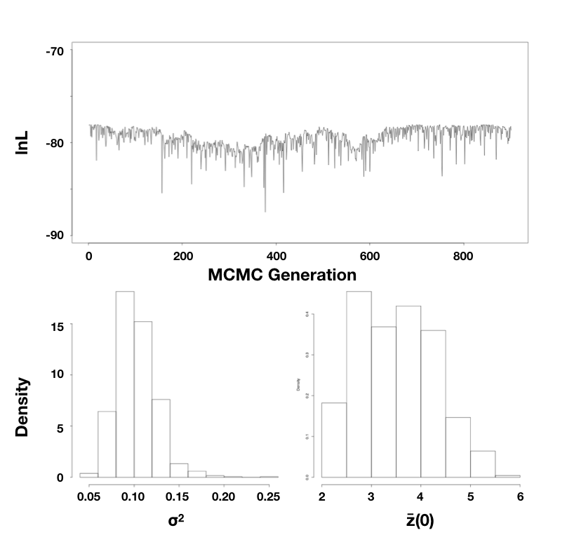
Using the mammal body size data, I ran an MCMC with 10,000 generations, discarding the first 1000 as burn-in. Sampling every 10 generations, I obtain parameter estimates of $\hat{\sigma}_{bayes}^2 = 0.10$ (95% credible interval: 0.066 − 0.15) and $\hat{\bar{z}}(0) = 3.5$ (95% credible interval: 2.3 − 5.3; Figure 4.5).

$Figure 4.5. Bayesian analysis of body size evolution in mammals. Figure shows the likelihood profile (A) and posterior distributions for model parameters \hat{\sigma}_{bayes}^2 (B) and \hat{\bar{z}}(0) (C). Image by the author, can be reused under a CC-BY-4.0 license.$

Figure shows the likelihood profile (A) and posterior distributions for model parameters $\hat{\sigma}_{bayes}^2$ (B) and $\hat{\bar{z}}(0)$ (C). Image by the author, can be reused under a CC-BY-4.0 license.

Note that the parameter estimates from all three approaches (REML, ML, and Bayesian) were similar. Even the confidence/credible intervals varied a little bit but were of about the same size in all three cases. All of the approaches above are mathematically related and should, in general, return similar results. One might place higher value on the Bayesian credible intervals over confidence intervals from the Hessian of the likelihood surface, for two reasons: first, the Hessian leads to an estimate of the CI under certain conditions that may or may not be true for your analysis; and second, Bayesian credible intervals reflect overall uncertainty better than ML confidence intervals (see chapter 2).