10.5: Tree topology, tree shape, and tree balance under a birth-death model

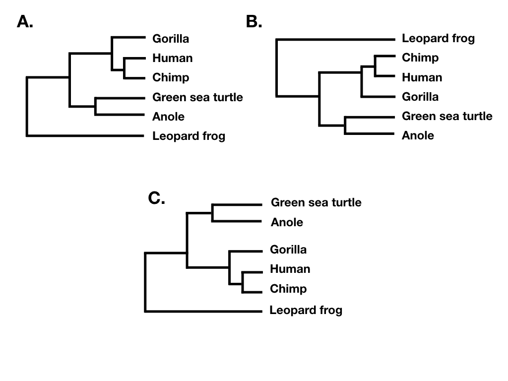
Tree topology summarizes the patterns of evolutionary relatedness among a group of species independent of the branch lengths of a phylogenetic tree. Two different trees have the same topology if they define the exact same set of clades. This is important because sometimes two trees can look very different and yet still have the same topology (e.g. Figure 10.6 A, B, and C).

Figure 10.6. Several phylogenetic trees showing different ways to plot the same tree topology. Image by the author, can be reused under a CC-BY-4.0 license.

Tree shape ignores both branch lengths and tree tip labels. For example, the two trees in figure 10.7 A and B have the same tree shape even though they share no tips in common. What they do share is that their nodes have the same patterns in terms of the number of descendants on each “side” of the bifurcation. By contrast, the phylogenetic tree in 10.7 C has a different shape. (Note that what I am calling tree shape is sometimes referred to as “unlabeled” tree topology; e.g. Felsenstein 2004).

Figure 10.7. Two different phylogenetic trees sharing the same tree shape (A and B), and one with a different shape (C). Image by the author, can be reused under a CC-BY-4.0 license.

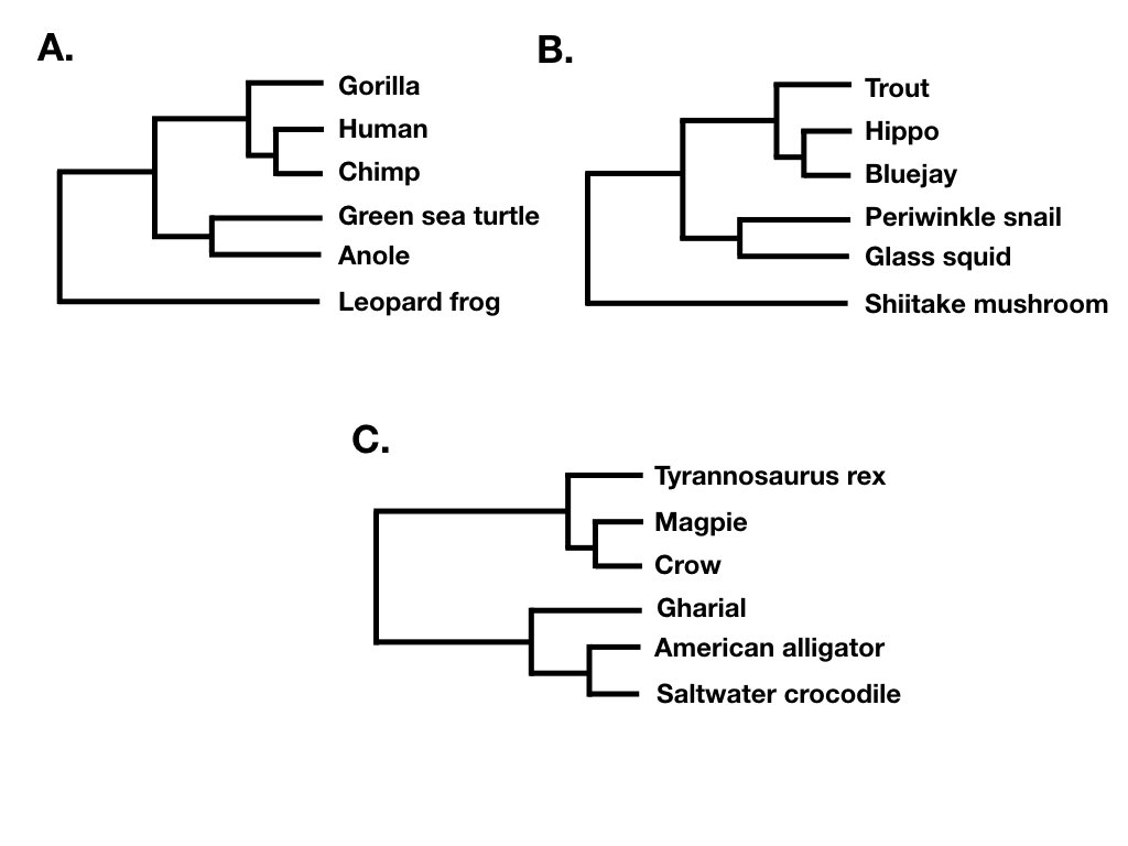
Finally, tree balance is a way of expressing differences in the number of descendants between pairs of sister lineages at different points in a phylogenetic tree. For example, consider the phylogenetic tree depicted in figure 10.7B. The deepest split in that tree separates a clade with five species (trout, hippo, bluejay, periwinkle snail, glass squid) from a clade with a single species (Shiitake mushroom), and so that node in the tree is unbalanced with a (5, 1) pattern. By contrast, the deepest split in 10.7C separates two clades of equal size. In that tree, the deepest node is balanced with a (3, 3) pattern. A number of approaches in macroevolution use balance at nodes and across whole trees to try to capture important evolutionary patterns.

We can start to understand these approaches by considering the balance of a single node n in a phylogenetic tree. There are two clades descended from this node; let’s call them a and b. We assume that the total number of species descended from the node N_total = N_a + N_b is constant and that neither N_a nor N_b is zero. An important result, first discussed by Farris (1976) for a pure-birth model, is that all possible numerical divisions of N_total into N_a + N_b are equally probable. For example, if N_total = 10, then all possible divisions: 1 + 9, 2 + 8, 3 + 7, 4 + 6, 5 + 5, 6 + 4, 7 + 3, 8 + 2, and 9 + 1 are all equally probable, so that each will be predicted to occur with a probability 1/9. Formally,

\[ p(N_a \mid N_{total})=\frac{1}{N_{total}-1} \label{19.17}\]

Note that there is a subtle difference between equation 10.2 above and some equations in the literature, e.g. Slowinski and Guyer (1993). This difference has to do with whether we label the two descendent clades, a and b, or not; if the clades are unlabeled, then there is no difference between 4+6 and 6+4, so that the probability that the largest clade, whichever it might be, has 6 species is twice what is given by my equation.

Equation 10.17 applies even if there is extinction, as long as both sister clades have the same speciation and extinction rates (Slowinski and Guyer 1993). This equation has been used to compare diversification rates between sister clades, either for a single pair or across multiple pairs (see Chapter 11).

Tree balance statistics provide a way of comparing numbers of taxa across all of the nodes in a phylogenetic tree simultaneously. There are a surprisingly large number of tree balance statistics, but all rely on summarizing information about the balance of each node across a whole tree. Colless’ index I_c (Colless 1982) is one of the simplest – and, perhaps, most commonly used – indices of tree balance. I_c is the sum of the difference in the number of tips subtended on each side of every node in the tree, standardized by the maximum that such a sum can achieve:

\[ I_C = \frac{\sum\limits_{all nodes} (N_L - N_R)}{(N-1)(N-2)/2} \label{10.18}\]

If the tree is perfectly balanced (only possible when N is some power of 2, e.g. 2, 4, 8, 16, etc.), then I_C = 0 (Figure 10.7C). By contrast, if the tree is completely pectinate, which means that each split in the tree contrasts a clade with 1 species with the rest of the species in the clade, then I_C = 1 (Figure 10.7A). All phylogenetic trees have values of I_C between 0 and 1 (Figure 10.7B).

Figure 10.8. A. a pectinate tree (I_C = 1); B. a random tree (0 < I_C < 1); C. A balanced tree (I_C = 0). Image by the author, can be reused under a CC-BY-4.0 license.

There are a number of other indices of phylogenetic tree balance (reviewed in Mooers and Heard 1997). All of these indices are used in a similar way: one can then compare the value of the tree index to what one might expect under a particular model of diversification, typically birth-death. In fact, since these indices focus on tree topology and ignore branch lengths, one can actually consider their general behavior under a set of equal-rates Markov (ERM) models. This set includes any model where birth and death rates are equal across all lineages in a phylogenetic tree at a particular time. ERM models include birth-death models as described above, but also encompass models where birth and/or death rates change through time.