10.2: The Birth-Death Model

Last updated
Save as PDF

Page ID: 21637

\( \newcommand{\vecs}[1]{\overset { \scriptstyle \rightharpoonup} {\mathbf{#1}} } \) \( \newcommand{\vecd}[1]{\overset{-\!-\!\rightharpoonup}{\vphantom{a}\smash {#1}}} \)\(\newcommand{\id}{\mathrm{id}}\) \( \newcommand{\Span}{\mathrm{span}}\) \( \newcommand{\kernel}{\mathrm{null}\,}\) \( \newcommand{\range}{\mathrm{range}\,}\) \( \newcommand{\RealPart}{\mathrm{Re}}\) \( \newcommand{\ImaginaryPart}{\mathrm{Im}}\) \( \newcommand{\Argument}{\mathrm{Arg}}\) \( \newcommand{\norm}[1]{\| #1 \|}\) \( \newcommand{\inner}[2]{\langle #1, #2 \rangle}\) \( \newcommand{\Span}{\mathrm{span}}\) \(\newcommand{\id}{\mathrm{id}}\) \( \newcommand{\Span}{\mathrm{span}}\) \( \newcommand{\kernel}{\mathrm{null}\,}\) \( \newcommand{\range}{\mathrm{range}\,}\) \( \newcommand{\RealPart}{\mathrm{Re}}\) \( \newcommand{\ImaginaryPart}{\mathrm{Im}}\) \( \newcommand{\Argument}{\mathrm{Arg}}\) \( \newcommand{\norm}[1]{\| #1 \|}\) \( \newcommand{\inner}[2]{\langle #1, #2 \rangle}\) \( \newcommand{\Span}{\mathrm{span}}\)\(\newcommand{\AA}{\unicode[.8,0]{x212B}}\)

A birth-death model is a continuous-time Markov process that is often used to study how the number of individuals in a population change through time. For macroevolution, these “individuals” are usually species, sometimes called "lineages" in the literature. In a birth-death model, two things can occur: births, where the number of individuals increases by one; and deaths, where the number of individuals decreases by one. We assume that no more than one new individual can form (or die) during any one event. In phylogenetic terms, that means that birth-death trees cannot have “hard polytomies” - each speciation event results in exactly two descendant species.

In macroevolution, we apply the birth-death model to species, and typically consider a model where each species has a constant probability of either giving birth (speciating) or dying (going extinct). We denote the per-lineage birth rate as λ and the per-lineage death rate as μ. For now we consider these rates to be constant, but we will relax that assumption later in the book.

We can understand the behavior of birth-death models if we consider the waiting time between successive speciation and extinction events in the tree. Imagine that we are considering a single lineage that exists at time t₀. We can think about the waiting time to the next event, which will either be a speciation event splitting that lineage into two (Figure 10.2A) or an extinction event marking the end of that lineage (Figure 10.2B). Under a birth-death model, both of these events follow a Poisson process, so that the expected waiting time to an event follows an exponential distribution (Figure 10.2C). The expected waiting time to the next speciation event is exponential with parameter λ, and the expected waiting time to the next extinction event exponential with parameter μ. [Of course, only one of these can be the next event. The expected waiting time to the next event (of any sort) is exponential with parameter λ + μ, and the probability that that event is speciation is λ/(μ + λ), extinction μ/(μ + λ)].

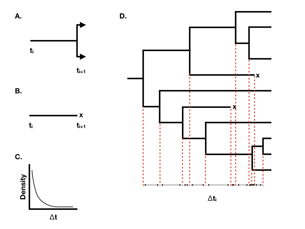
Figure 10.2. Illustration of the basic properties of birth-death models. A. Waiting time to a speciation event; B. Waiting time to an extinction event; C. Exponential distribution of waiting times until the next event; D. A birth-death tree with waiting times, with x denoting extinct taxa. Image by the author, can be reused under a CC-BY-4.0 license.

When we have more than one lineage “alive” in the tree at any time point, then the waiting time to the next event changes, although its distribution is still exponential. In general, if there are N(t) lineages alive at time t, then the waiting time to the next event follows an exponential distribution with parameter N(t)(λ + μ), with the probability that that event is speciation or extinction the same as given above. You can see from this equation that the rate parameter of the exponential distribution gets larger as the number of lineages increases. This means that the expected waiting times across all lineages get shorter and shorter as more lineages accumulate.

Using this approach, we can grow phylogenetic trees of any size (Figure 10.2D).

We can derive some important properties of the birth-death process on trees. To do so, it is useful to define two additional parameters, the net diversification rate (r) and the relative extinction rate (ϵ):

\[r = λ − μ \label{10.A}\]

\[ \epsilon = \frac{\mu}{\lambda} \lable{10.1B}\]

These two parameters simplify some of the equations below, and are also commonly encountered in the literature.

To derive some general properties of the birth-death model, we first consider the process over a small interval of time, Δt. We assume that this interval is so short that it contains at most a single event, either speciation or extinction (the interval might also contain no events at all). The probability of speciation and extinction over the time interval can be expressed as:

\[Pr_{speciation} = N(t)λΔt \label{10.2A}\]

\[Pr_{extinction} = N(t)μΔt \label{10.2B}\]

We now consider the total number of living species at some time t, and write this as N(t). It is useful to think about the expected value of N(t) under a birth-death model [we consider the full distribution of N(t) below]. The expected value of N(t) after a small time interval Δt is:

\[N(t + Δt)=N(t)+N(t)λΔt − N(t)μΔt \label{10.3}\]

We can convert this to a differential equation by subtracting N(t) from both sides, then dividing by Δt and taking the limit as Δt becomes very small:

\[dN/dt = N(λ − μ) \label{10.4}\]

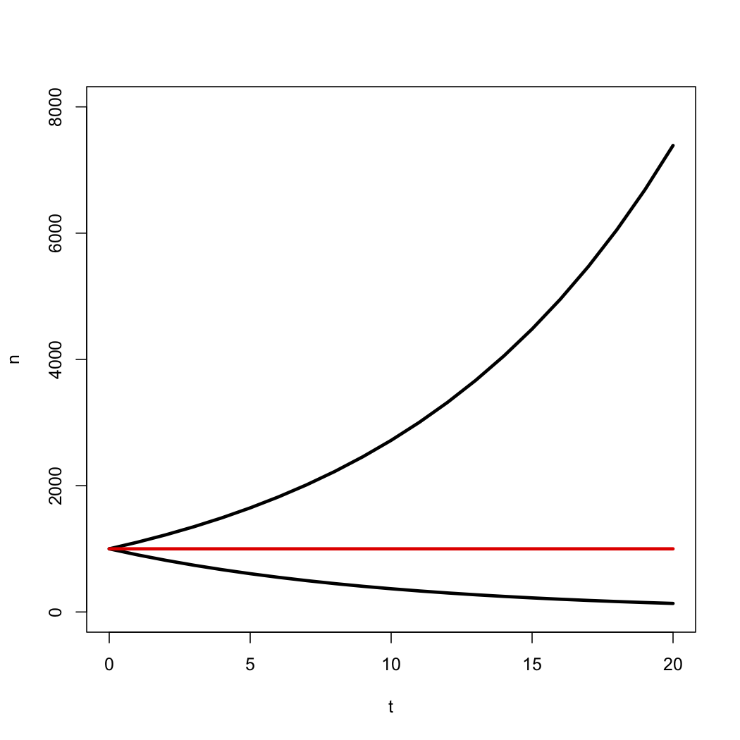
We can solve this differential equation if we set a boundary condition that N(0)=n₀; that is, at time 0, we start out with n₀ lineages. We then obtain:

\[N(t)=n_0e^{λ − μ}t = n_0e^{rt} \label{10.5}\]

This deterministic equation gives us the expected value for the number of species through time under a birth-death model. Notice that the number of species grows exponentially through time as long as λ > μ, i.e. r > 0, and decays otherwise (Figure 10.3).

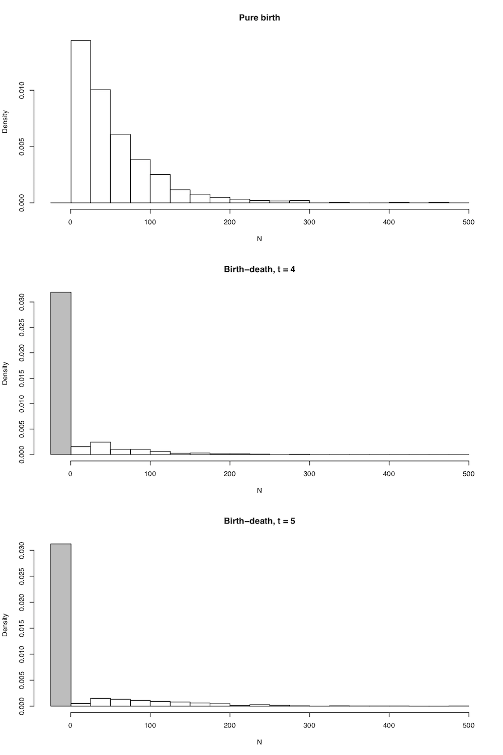
Figure 10.3. Expected number of species under a birth-death model with r=\lambda-\mu > 0 (top line), r = 0 (middle line), and r < 0 (bottom line). In each case the starting number of species was n_0 = 1000. Image by the author, can be reused under a CC-BY-4.0 license. — Figure 10.3. Expected number of species under a birth-death model with r = λ − μ > 0 (top line), r = 0 (middle line), and r < 0 (bottom line). In each case the starting number of species was n₀ = 1000. Image by the author, can be reused under a CC-BY-4.0 license.

We are also interested in the stochastic behavior of the model – that is, how much should we expect N(t) to vary from one replicate to the next? We can calculate the full probability distribution for N(t), which we write as p_n(t)=Pr[N(t)=n] for all n ≥ 0, to completely describe the birth-death model’s behavior. To derive this probability distribution, we can start with a set of equations, one for each value of n, to keep track of the probabilities of n lineages alive at time t. We will denote each of these as p_n(t) (there are an infinite set of such equations, from p₀ to p_∞). We can then write a set of difference equations that describe the different ways that one can reach any state over some small time interval Δt. We again assume that Δt is sufficiently small that at most one event (a birth or a death) can occur. As an example, consider what can happen to make n = 0 at the end of a certain time interval. There are two possibilities: either we were already at n = 0 at the beginning of the time interval and (by definition) nothing happened, or we were at n = 1 and the last surviving lineage went extinct. We write this as:

(eq. 10.6)

p₀(t + Δt)=p₁(t)μΔt + p₀(t)

Similarly, we can reach n = 1 by either starting with n = 1 and having no events, or going from n = 2 via extinction.

(eq. 10.7)

p₁(t + Δt)=p₁(t)(1 − (λ + μ))Δt + p₂(t)2μΔt

Finally, any for n > 1, we can reach the state of n lineages in three ways: from a birth (from n − 1 to n), a death (from n + 1 to n), or neither (from n to n).

(eq. 10.8)

p_n(t + Δt)=p_n − 1(t)(n − 1)λΔt + p_n + 1(t)(n + 1)μΔt + p_n(t)(1 − n(λ + μ))Δt

We can convert this set of difference equations to differential equations by subtracting p_n(t) from both sides, then dividing by Δt and taking the limit as Δt becomes very small. So, when n = 0, we use 10.6 to obtain:

(eq. 10.9)

dp₀(t)/dt = μp₁(t)

From 10.7:

(eq. 10.10)

dp₁(t)/dt = 2μp₂(t)−(λ − μ)p₁(t)

and from 10.8, for all n > 1:

(eq. 10.11)

dp_n(t)/dt = (n − 1)λp_n − 1(t)+(n + 1)μp_n + 1(t)−n(λ + μ)p_n(t)

We can then solve this set of differential equations to obtain the probability distribution of p_n(t). Using the same boundary condition, N(0)=n₀, we have p₀(t)=1 for n = n₀ and 0 otherwise. Then, we can find the solution to the differential equations 10.9, 10.10, and 10.11. The derivation of the solution to this set of differential equations is beyond the scope of this book (but see Kot 2001 for a nice explanation of the mathematics). A solution was first obtained by Bailey (1964), but I will use the simpler equivalent form from Foote et al. (1999). For p₀(t) – that is, the probability that the entire lineage has gone extinct at time t – we have:

(eq. 10.12)

p₀(t)=α₀ⁿ

And for all n ≥ 1:

(eq. 10.13)

\[ p_n(t) = \sum\limits_{j=1}^{min(n_0,n)} \binom{n_0}{j} \binom{n-1}{j-1} \alpha^{n_0 - j} \beta^{n-j} [(1-\alpha)(1-\beta)]^j \]

Where α and β are defined as:

(eq. 10.14)

\[ \alpha=\frac{\epsilon (e^rt-1)}{(e^rt-\epsilon)} \]

\[ \beta =\frac{(e^rt-1)}{(e^rt-\epsilon)} \]

α is the probability that any particular lineage has gone extinct before time t.

Note that when n₀ = 1 – that is, when we start with a single lineage - equations 10.12 and 10.13 simplify to (Raup 1985):

(eq. 10.15)

p₀(t)=α

And for all n ≥ 1:

(eq. 10.16)

p_n(t)=(1 − α)(1 − β)β^i − 1

In all cases the expected number of lineages in the tree is exactly as stated above in equation (10.5), but now we have the full probability distribution of the number of lineages given n₀, t, λ, and μ. A few plots capture the general shape of this distribution (Figure 10.4).

Figure 10.4. Probability distributions of N(t) under A. pure birth, B. birth death after a short time, and C. birth-death after a long time. Image by the author, can be reused under a CC-BY-4.0 license.

There are quite a few comparative methods that use clade species richness and age along with the distributions defined in 10.14 and 10.15 to make inferences about clade diversification rates (see chapter 11).