7.3: The Mk Model

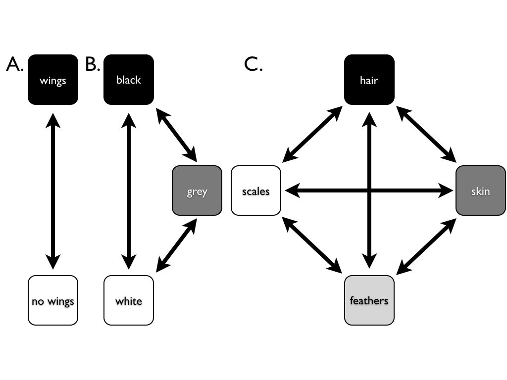
The most basic model for discrete character evolution is called the Mk model. First developed for trait data by Pagel (1994; although the name Mk comes from Lewis 2001). The Mk model is a direct analogue of the Jukes-Cantor (JC) model for sequence evolution. The model applies to a discrete character having k unordered states. Such a character might have k = 2, k = 3, or even more states. Evolution involves changing between these k states (Figure 7.3).

Figure 7.3. Examples of discrete characters with (A) k = 2, (B) k = 3, and (C) k = 4 states. Image by the author, can be reused under a CC-BY-4.0 license.

The basic version of the Mk model assumes that transitions among these states follow a Markov process. This means that the probability of changing from one state to another depends only on the current state, and not on what has come before. For example, it makes no difference if a lineage has just evolved the trait of “feathers,” or whether they have had feathers for millions of years – the probability of evolving a different character state is the same in both cases. The basic Mk model also assumes that every state is equally likely to change to any other state.

For the basic Mk model, we can denote the instantaneous rate of change between states using the parameter q. In general, q_ij is called the instantaneous rate between character states i and j. It is defined as the limit of the rate measured over very short time intervals¹.

Again, for the basic Mk model, instantaneous rates between all pairs of characters are equal; that is, q_ij = q_mn for all i ≠ j and m ≠ n.

We can summarize general Markov models for discrete characters using a transition rate matrix (Lewis 2001):

\[ \mathbf{Q} = \begin{bmatrix} -d_1 & q_{12} & \dots & q_{1k} \\ q_{21} & -d_2 & \dots & q_{2k} \\ \vdots & \vdots & \ddots & \vdots\\ q_{k1} & q{k2} & \dots & -d_k \\ \end{bmatrix} \label{7.1}\]

Note that the instantaneous rates are only entered into the off-diagonal parts of the matrix. Along the diagonal, these matrices always have a set of negative numbers. For any Q matrix, the sum of all the elements in each row is zero – a necessary condition for a transition rate matrix. Because of this, each negative number has a value, d_i, equal to the sum of all of the other numbers in the row. For example,

\[ d_1 = \sum_{i=2}^{k} q_{1i} \label{7.2}\]

For a two-state Mk model, k = 2 and rates are symmetric so that q₁₂ = q₂₁. In this case, we can write the transition rate matrix as:

\[ \mathbf{Q} = \begin{bmatrix} -q & q \\ q & -q \\ \end{bmatrix} \label{7.3}\]

Likewise, for k = 3, the transition rate matrix is:

\[ \mathbf{Q} = \begin{bmatrix} -2 q & q & q\\ q & -2 q & q\\ q & q & -2 q\\ \end{bmatrix} \label{7.4}\]

In general, the k-state transition matrix for a basic Mk model is:

\[ \mathbf{Q} = \begin{bmatrix} 1-k & 1 & \dots & 1\\ 1 & 1-k & \dots & 1\\ \vdots & \vdots & \ddots & \vdots\\ 1 & 1 & \dots & 1\\ \end{bmatrix} \label{7.5}\]

Once we have this transition rate matrix, we can calculate the probability distribution of trait states after any time interval t using the equation (Lewis 2001):

\[\textbf{P}(t)=e^{\textbf{Q}t} \label{7.6}\]

This equation looks simple, but calculating P(t) involves matrix exponentiation – raising e to a power defined by a matrix. This calculation is substantially different from raising e to the power defined by each element of a matrix². The result is a matrix, P, of transition probabilities. Each element in this matrix (p_ij) gives the probability that starting in state i you will end up in state j over that time interval t. For the standard Mk model, there is a general solution to this equation:

\[ \begin{array}{l} p_{ii}(t) = \frac{1}{k} + \frac{k-1}{k} e^{-kqt} \\ p_{ij}(t) = \frac{1}{k} - \frac{1}{k} e^{-kqt} \\ \end{array} \label{7.7}\]

In particular, when k = 2,

\[ \begin{array}{l} p_{ii}(t) = \frac{1}{k} + \frac{k-1}{k} e^{-kqt} = \frac{1}{2} + \frac{2-1}{2}e^{-2qt}=\frac{1+e^{-2qt}}{2} \\ p_{ij}(t) = \frac{1}{k} - \frac{1}{k} e^{-kqt} = \frac{1}{2} - \frac{1}{2}e^{-2qt}=\frac{1-e^{-2qt}}{2} \\ \end{array} \label{7.8}\]

If we consider what happens when time gets very large in these equations, we see an interesting pattern. Any term that has e^−t in it gets closer and closer to zero as t increases. Because of this, for all values of k, each p_ij(t) converges to a constant value, 1/k. This is the stationary distribution of character states, π, defined as the equilibrium frequency of character states if the process is run many times for a long enough time period. In general, the stationary distribution of an Mk model is:

\[ \pi = \begin{bmatrix} 1/k & 1/k & \dots & 1/k\\ \end{bmatrix} \label{7.9}\]

In the case of \(k = 2\),

\[ \pi = \begin{bmatrix} 1/2 & 1/2 \\ \end{bmatrix} \label{7.10}\]