4.2: Estimating Rates using Independent Contrasts

Last updated
Save as PDF

Page ID: 21596

$ \newcommand{\vecs}[1]{\overset { \scriptstyle \rightharpoonup} {\mathbf{#1}} } $ $ \newcommand{\vecd}[1]{\overset{-\!-\!\rightharpoonup}{\vphantom{a}\smash {#1}}} $$\newcommand{\id}{\mathrm{id}}$ $ \newcommand{\Span}{\mathrm{span}}$ $ \newcommand{\kernel}{\mathrm{null}\,}$ $ \newcommand{\range}{\mathrm{range}\,}$ $ \newcommand{\RealPart}{\mathrm{Re}}$ $ \newcommand{\ImaginaryPart}{\mathrm{Im}}$ $ \newcommand{\Argument}{\mathrm{Arg}}$ $ \newcommand{\norm}[1]{\| #1 \|}$ $ \newcommand{\inner}[2]{\langle #1, #2 \rangle}$ $ \newcommand{\Span}{\mathrm{span}}$ $\newcommand{\id}{\mathrm{id}}$ $ \newcommand{\Span}{\mathrm{span}}$ $ \newcommand{\kernel}{\mathrm{null}\,}$ $ \newcommand{\range}{\mathrm{range}\,}$ $ \newcommand{\RealPart}{\mathrm{Re}}$ $ \newcommand{\ImaginaryPart}{\mathrm{Im}}$ $ \newcommand{\Argument}{\mathrm{Arg}}$ $ \newcommand{\norm}[1]{\| #1 \|}$ $ \newcommand{\inner}[2]{\langle #1, #2 \rangle}$ $ \newcommand{\Span}{\mathrm{span}}$$\newcommand{\AA}{\unicode[.8,0]{x212B}}$

The information required to estimate evolutionary rates is efficiently summarized in the early (but still useful) phylogenetic comparative method of independent contrasts (Felsenstein 1985). Independent contrasts summarize the amount of character change across each node in the tree, and can be used to estimate the rate of character change across a phylogeny. There is also a simple mathematical relationship between contrasts and maximum-likelihood rate estimates that I will discuss below.

We can understand the basic idea behind independent contrasts if we think about the branches in the phylogenetic tree as the historical “pathways” of evolution. Each branch on the tree represents a lineage that was alive at some time in the history of the Earth, and during that time experienced some amount of evolutionary change. We can imagine trying to measure that change initially by comparing sister taxa. We can compare the trait values of the two sister taxa by finding the difference in their trait values, and then compare that to the total amount of time they have had to evolve that difference. By doing this for all sister taxa in the tree, we will get an estimate of the average rate of character evolution ( 4.1A). But what about deeper nodes in the tree? We could use other non-sister species pairs, but then we would be counting some branches in the tree of life more than once (Figure 4.1B). Instead, we use a “pruning algorithm,” (Felsenstein 1985, Felsenstein (2004)) chopping off pairs of sister taxa to create a smaller tree (Figure 4.1C). Eventually, all of the nodes in the tree will be trimmed off – and the algorithm will finish. Independent contrasts provides a way to generalize the approach of comparing sister taxa so that we can quantify the rate of evolution throughout the whole tree.

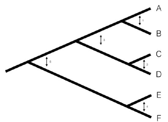
Figure 4.1. Pruning algorithm that can be used to identify five independent contrasts for a tree with six species (following Felsenstein 1985). The numbered order in this figure is only one of several possibilities that work; one can also prune the tree in the order 1, 2, 4, 3, 5 and get identical results. Image by the author, can be reused under a CC-BY-4.0 license.

A more precise algorithm describing how Phylogenetic Independent Contrasts (PICs) are calculated is provided in Box 4.2, below (from Felsenstein 1985). Each contrast can be described as an estimate of the direction and amount of evolutionary change across the nodes in the tree. PICs are calculated from the tips of the tree towards the root, as differences between trait values at the tips of the tree and/or calculated average values at internal nodes. The differences themselves are sometimes called “raw contrasts” (Felsenstein 1985). These raw contrasts will all be statistically independent of each other under a wide range of evolutionary models. In fact, as long as each lineage in a phylogenetic tree evolves independently of every other lineage, regardless of the evolutionary model, the raw contrasts will be independent of each other. However, people almost never use raw contrasts because they are not identically distributed; each raw contrast has a different expected distribution that depends on the model of evolution and the branch lengths of the tree. In particular, under Brownian motion we expect more change on longer branches of the tree. Felsenstein (1985) divided the raw contrasts by their expected standard deviation under a Brownian motion model, resulting in standardized contrasts. These standardized contrasts are, under a BM model, both independent and identically distributed, and can be used in a variety of statistical tests. Note that we must assume a Brownian motion model in order to standardize the contrasts; results derived from the contrasts, then, depend on this Brownian motion assumption.

Box 4.2: Algorithm for Phylogenetic Independent Contrasts

One can calculate PICs using the algorithm from Felsenstein (1985). I reproduce this algorithm below. Keep in mind that this is an iterative algorithm – you repeat the five steps below once for each contrast, or n − 1 times over the whole tree (see Figure 4.1C as an example).

Find two tips on the phylogeny that are adjacent (say nodes i and j) and have a common ancestor, say node k. Note that the choice of which node is i and which is j is arbitrary. As you will see, we will have to account for this “arbitrary direction” property of PICs in any analyses where we use them to do certian analyses!
Compute the raw contrast, the difference between their two tip values:\[c_{ij} = x_i − x_j \label{4.1}\]

Under a Brownian motion model, c_ij has expectation zero and variance proportional to v_i + v_j.

Calculate the standardized contrast by dividing the raw contrast by its variance \[ s_{ij} = \frac{c_{ij}}{v_i + v_j} = \frac{x_i - x_j}{v_i + v_j} \label{4.2}\[

Under a Brownian motion model, this contrast follows a normal distribution with mean zero and variance equal to the Brownian motion rate parameter σ².

Remove the two tips from the tree, leaving behind only the ancestor k, which now becomes a tip. Assign it the character value: \[ x_k = \frac{(1/v_i)x_i+(1/v_j)x_j}{1/v_1+1/v_j} \label{4.3}\[
- It is worth noting that x_k is a weighted average of x_i and x_j, but does not represent an ancestral state reconstruction, since the value is only influenced by species that descend directly from that node and not other relatives.
Lengthen the branch below node k by increasing its length from v_k to v_k + v_iv_j/(v_i + v_j). This accounts for the uncertainty in assigning a value to x_k.

As mentioned above, we can apply the algorithm of independent contrasts to learn something about rates of body size evolution in mammals. We have a phylogenetic tree with branch lengths as well as body mass estimates for 49 species (Figure 4.2). If we ln-transform mass and then apply the method above to our data on mammal body size, we obtain a set of 48 standardized contrasts. A histogram of these contrasts is shown as Figure 4.2 (data from from Garland 1992).

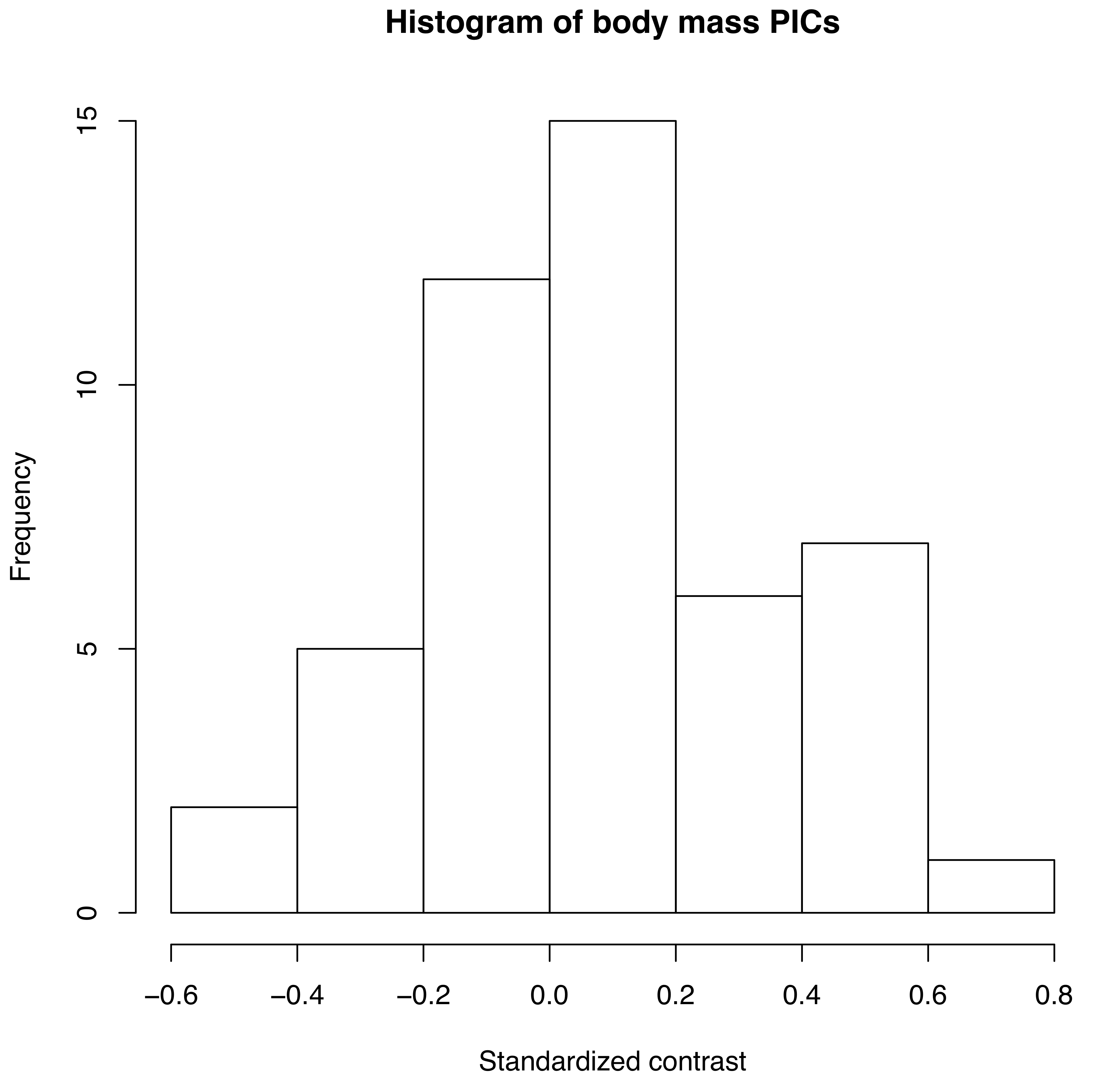
Figure 4.2. Histogram of PICs for ln-transformed mammal body mass on a phylogenetic tree with branch lengths in millions of years (data from Garland 1992). Image by the author, can be reused under a CC-BY-4.0 license.

Note that each contrast is an amount of change, x_i − x_j, divided by a branch length, v_i + v_j, which is a measure of time. Thus, PICs from a single trait can be used to estimate σ², the rate of evolution under a Brownian model. The PIC estimate of the evolutionary rate is:

\[ \hat{\sigma}_{PIC}^2 = \frac{\sum{s_{ij}^2}}{n-1} \label{4.4}\]

That is, the PIC estimate of the evolutionary rate is the average of the n − 1 squared contrasts. This sum is taken over all s_ij, the standardized independent contrast across all (i, j) pairs of sister branches in the phylogenetic tree. For a fully bifurcating tree with n tips, there are exactly n − 1 such pairs. If you are statistically savvy, you might note that this formula looks a bit like a variance. In fact, if we state that the contrasts have a mean of 0 (which they must because Brownian motion has no overall trends), then this is a formula to estimate the variance of the contrasts.

If we calculate the mean sum of squared contrasts for the mammal body mass data, we obtain a rate estimate of $\hat{\sigma}_{PIC}^2$ = 0.09. We can put this into words: if we simulated mammalian body mass evolution under this model, we would expect the variance across replicated runs to increase by 0.09 per million years. Or, in more concrete terms, if we think about two lineages diverging from one another for a million years, we can draw changes in ln-body mass for both of them from a normal distribution with a variance of 0.09. Their difference, then, which is the amount of expected divergence, will be normal with a variance of 2 ⋅ 0.09 = 0.18. Thus, with 95% confidence, we can expect the two species to differ maximally by two standard deviations of this distribution, $2 \cdot \sqrt{0.18} = 0.85$. Since we are on a log scale, this amount of change corresponds to a factor of e^2.68 = 2.3, meaning that one species will commonly be about twice as large (or small) as the other after just one million years.