16.7: Multiple resource phase space

As the next step, consider the case of two essential resources. This can be done mathematically following the approach we used earlier for a single resource.

Call the two resources \(R_A\) and \(R_B\). Suppose that of the total of these two resources used by Species 1, a proportion \(p_1\) is Resource A and therefore a proportion \(q_1\,=\,1−p_1\) is Resource B. Likewise, for Species 2 a proportion \(p_2\) is Resource A and \(q_2\,=\,1−p_2\) is Resource B.

This is confusing, so for a clarifying example, suppose \(R_A\) is phosphate, PO₄, and \(R_B\) is silicate, SiO₂, both essential to two species of algae in a waterway. Take Species 1 to be an Asterionella species and Species 2 to be a Cyclotella species, as in a pioneering study by David Tilman (1977). In this case, Species 1 needs phosphate and silicate resources in about a 1:99 ratio, while Species 2 needs them in about a 6:94 ratio. If silicate is low, Species 1 will thus suffer first, since it needs a larger proportion of it, while Species 2 will suffer first if phosphate is low, for the related reason. Here it would be \(p_1\,=\,0.01,\,q_1\,=\,1−p_1\,=\,0.99\) for the use of Resources A and B by Species 1, and \(p_2\,=\,0.06,\,q_1\,=\,1−p_1\,=\,0.94\) for use by Species 2.

With \(u_1\) being the total amount of resource tied up by each individual of Species 1, \(p_1u_1\) will be the amount of Resource A tied up by Species 1 and \(q_1u_1\) the amount of Resource B tied up the same way. Similarly, \(p_2u_2\) will be the amount of Resource A tied up by each individual of Species 2 and \(q_2u_2\) the amount of Resource B. Also, assume as before that the resources under consideration disappear from the environment when they are taken up by individuals newly born, are released immediately when individuals die.

With this in mind, the resources remaining at any time, as functions of the maximum resource and the abundance of each species, will be

\[R_A\,=\,R_{Amax}\,-\,p_1u_1N_1\,-\,p_2u_2N_2\]

\[R_A\,=\,R_{Bmax}\,-\,q_1u_1N_1\,-\,q_2u_2N_2\]

Suppose that populations of Species 1 and 2 grow based on which resource is closest to the \(R^{\ast}\) experienced by that species for the resource. This can be represented by the “min” function, min(\(a,b\)), which selects the smaller of two values. For example, min(200,10) = 10, min(−200,10) = −200. Now the two-species, two-resource growth equations, generalizing the single-species, single-resource growth in Equation 16.1.1, are

\(\frac{1}{N_1}\frac{dN_1}{dt}\,=\,m_1\,min(R_A\,-\,R_{1A}^{\ast},\,R_B\,-\,R_{1B}^{\ast})\)

\(\frac{1}{N_2}\frac{dN_2}{dt}\,=\,m_2\,min(R_A\,-\,R_{2A}^{\ast},\,R_B\,-\,R_{2B}^{\ast})\)

This could be refined, so that the growth rates \(m_1\) and \(m_2\) would depend on which resource was limiting, but this does not matter in the present analysis. If the species are similar enough and the resource level is such that they are limited by the same resource, one will tend to be competitively excluded, as in the previous section. But if the two species are quite different, they can be limited by different resources and the equations can be simplified.

\[\frac{1}{N_1}\frac{dN_1}{dt}\,=\,m_1(R_A\,-\,R_{1A}^{\ast})\]

\[\frac{1}{N_2}\frac{dN_2}{dt}\,=\,m_2(R_B\,-\,R_{2B}^{\ast})\]

Some algebra will reveal the basic properties. If you substitute the expressions for \(R_1\) and \(R_2\) from Equations 16.6.1 and 16.6.2 into Equations 16.6.3 and 16.6.4 you will get

\[\frac{1}{N_1}\frac{dN_1}{dt}\,=\,m_1(R_{Amax}\,-\,p_1u_1N_1\,-\,p_2U_2N_2\,-\,R_{1A}^{\ast})\]

\[\frac{1}{N_2}\frac{dN_2}{dt}\,=\,m_2(R_{Bmax}\,-\,q_1u_1N_1\,-\,q_2u_2N_2\,-\,R_{2B}^{\ast})\]

Now if you expand, collect, and rearrange terms, you get this equivalent form:

\[\frac{1}{N_1}\frac{dN_1}{dt}\,=\,m_1(R_{Amax}\,-\,R_{1A}^{\ast})\,-\,m_1p_1u_1N_1\,-\,m_1p_2u_2N_2\]

\[\frac{1}{N_2}\frac{dN_2}{dt}\,=\,m_2(R_{Bmax}\,-\,R_{2B}^{\ast})\,-\,m_2q_2u_2N_2\,-\,m_2q_1u_1N_1\]

Notice that, again, a mechanistic model with measurable parameters is just the general ecological RSN model in disguise.

The RSN formulation can expose the possibilities of two-resource situations in phase space. The isoclines are Equations 16.5.5 and 16.5.6 of this chapter, with slopes −\(s_{1,1}/s_{1,2}\) and −\(s_{2,1}/s_{2,2}\) for Species 1 and 2, respectively.

These two slopes can be written in terms of the resource. With the values for \(s_{i,j}\) from Equations 16.6.7 and 16.6.8 \((s_{1,1}\,=\,−m_1p_1u_1,\,s_{1,2}\,=\,−m_1p_2u_2,\,s_{2,1}\,=\,−m_2q_1u_1,\) and \(s_{2,2}\,=\,−m_2q_2u_2\)), the slopes of the isoclines become

\(\frac{s_{1,1}}{s_{1,2}}\,=\,\frac{-m_1p_1u_1}{-m_1p_2u_2}\,=\,\frac{u_1}{u_2}\frac{p_1}{p_2}\)

\(\frac{s_{1,1}}{s_{1,2}}\,=\,\frac{-m_1p_1u_1}{-m_1p_2u_2}\,=\,\frac{u_1}{u_2}\frac{1-p_1}{1-p_2}\)

First notice that if the two species use the two resources in equal proportions (if \(p_1\,=\,p_2\)), both slopes become \(u_1/u_2\). The slopes are parallel, as in the single-resource case in Figures 16.5.1 through 16.5.4. Therefore, if two species use two different resources identically—that is, in equal proportions— they do not coexist. Coexistence requires some difference in how they use resources.

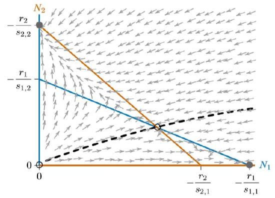
However, using the resources differently does not guarantee coexistence. Depending on their \(p\)’s and \(q\)’s, one isocline could still enclose the other completely. Figure \(\PageIndex{1}\) has the same properties as Figure 16.5.4. Everywhere below the red isocline, Species 2 will increase, including the broad band between the red and blue isoclines where Species 1 will decrease.

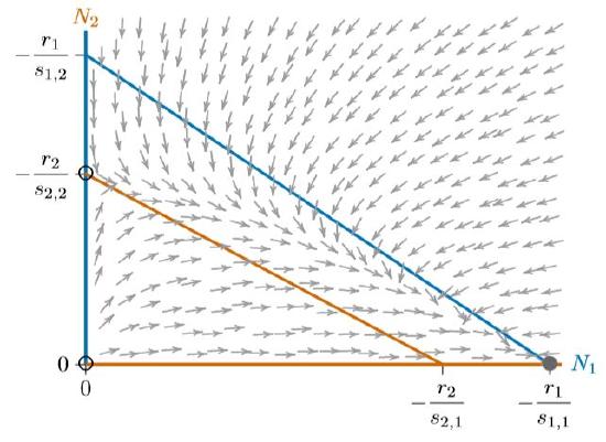
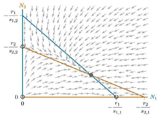
If the blue and red isoclines are reversed, the result is similar, but with Species 1 excluding Species 2. Figure \(\PageIndex{2}\) shows this, with the arrows reversed as Species 1 increases everywhere below the blue isocline, including the broad band between the isoclines where Species 2 decreases.

Figure \(\PageIndex{1}\). Two species using resources differently, with Species 2 excluding Species 1. (\(r_1\,=\,0.75,\,r_2\,=\,0.65,\,s_{12}\,= \,−1.875,\,s_{21}\,=\, −0.666,\,s_{11}=s_{22}=−1\))

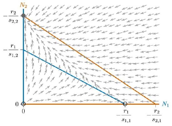
In all three cases, from Figures 16.5.4 to \(\PageIndex{2}\), the system has three equilibria—at the origin (0,0), where both species are absent, at the carrying capacity \(K_1\) for Species 1 alone (−\(r_1/s_{1,1}\),0), and at the carrying capacity \(K_2\) for Species 2 alone (0,\(−r_2/s_{2,2}\)). The origin is unstable and only one of the other two equilibria is stable, depending on which isocline encloses the other.

Figure \(\PageIndex{2}\). The opposite of Figure \(\PageIndex{1}\), with Species 1 excluding Species 2. (\(r_1\,=0.975,\,r_2\,=0.4,\,s_{12}\,=−1.5,\,s_{21}\,=−0.533,\, s_{11}=s_{22}=−1\)).

Figures \(\PageIndex{1}\) and \(\PageIndex{2}\) can be combined to give each species a chance to exclude the other, depending on circumstances. This means not allowing one isocline to completely enclose the other, as in Figure \(\PageIndex{3}\). Intersecting isoclines introduce a fourth equilibrium at the interior of the phase space. This equilibrium is unstable, marked with an open circle, and the two equilibria for the individual species, on the axes, are stable. They are no longer “globally stable,” however, since only local regions of the phase space lead to either of them.

Figure \(\PageIndex{3}\). Isoclines intersecting in a way that allows each species to exclude the other, depending on starting conditions.

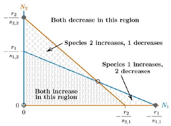
Depending on where the populations start, one of the two species will exclude the other. A curve called a “separatrix,” dividing these starting points according to which species will exclude the other, is shown with the dashed black line in Figure \(\PageIndex{4}\). That separatrix corresponds to a long curved ridge in any surface above the phase space, as described in Chapter 10. It necessarily passes through the unstable interior equilibrium. Here it is a simple curve, though in some cases (such as the Mandelbrot system, not representing competition), related curves can be infinitely complex.

Copy and paste image here

Figure \(\PageIndex{4}\). Flow in the bistable system of Figure \(\PageIndex{3}\). The black dashed line is a separatrix, dividing the phase space into regions that reach one stable equilibrium or the other. (\(r_1=0.975,\,r_2=0.65,\,s_{12}=−2.437,\,s{21}=−0.866,\,s_{11}=s_{22}=−1\)).

Finally, the isoclines can intersect in the opposite way, as in Figure \(\PageIndex{5}\). In this case, neither species has any region where its isocline encloses the other, as seen in each of the phase spaces of Figures 16.5.4 through \(\PageIndex{4}\). What will happen when neither species can exclude the other in any part of the phase space? They are forced to coexist. The individual equilibria on the axes become unstable and the interior equilibrium becomes stable—indeed, globally stable.

Figure \(\PageIndex{5}\). Isoclines intersecting at a globally stable coexistence. (\(r_1 =0.75,\,r_2=0.4,\,s_{12}\,=−1.153,\,s_{21}=−0.410, s_{11}=s_{22}=−1\)).

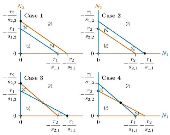
In summary, the isoclines in competitive systems have four different configurations, as in Figure \(\PageIndex{6}\). Cases 1 and 2 can represent competition for a single resource or, equivalently, competition for two different resources that the two species handle identically. One of the two is a superior competitor that excludes the other. Case 3 is “bistable,” where either of the species can exclude the other, depending on how the system starts out. Finally, Case 4 is globally stable, where neither species can exclude the other, and stable coexistence prevails. Cases 3 and 4 can represent competition for two different resources.

Figure \(\PageIndex{6}\). Case 1: Species 2 excludes Species 1. Case 2: Species 1 excludes Species 2. Case 3: one excludes the other, depending on starting conditions. Case 4: both species coexist.