7.4: Sensitive Dependence

Last updated
Save as PDF

Page ID: 25459

\( \newcommand{\vecs}[1]{\overset { \scriptstyle \rightharpoonup} {\mathbf{#1}} } \) \( \newcommand{\vecd}[1]{\overset{-\!-\!\rightharpoonup}{\vphantom{a}\smash {#1}}} \)\(\newcommand{\id}{\mathrm{id}}\) \( \newcommand{\Span}{\mathrm{span}}\) \( \newcommand{\kernel}{\mathrm{null}\,}\) \( \newcommand{\range}{\mathrm{range}\,}\) \( \newcommand{\RealPart}{\mathrm{Re}}\) \( \newcommand{\ImaginaryPart}{\mathrm{Im}}\) \( \newcommand{\Argument}{\mathrm{Arg}}\) \( \newcommand{\norm}[1]{\| #1 \|}\) \( \newcommand{\inner}[2]{\langle #1, #2 \rangle}\) \( \newcommand{\Span}{\mathrm{span}}\) \(\newcommand{\id}{\mathrm{id}}\) \( \newcommand{\Span}{\mathrm{span}}\) \( \newcommand{\kernel}{\mathrm{null}\,}\) \( \newcommand{\range}{\mathrm{range}\,}\) \( \newcommand{\RealPart}{\mathrm{Re}}\) \( \newcommand{\ImaginaryPart}{\mathrm{Im}}\) \( \newcommand{\Argument}{\mathrm{Arg}}\) \( \newcommand{\norm}[1]{\| #1 \|}\) \( \newcommand{\inner}[2]{\langle #1, #2 \rangle}\) \( \newcommand{\Span}{\mathrm{span}}\)\(\newcommand{\AA}{\unicode[.8,0]{x212B}}\)

alt Sensitive Dependence.JPG

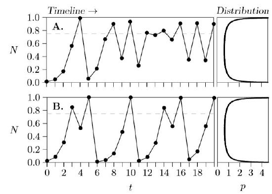
Figure \(\PageIndex{1}\). Sensitive dependence on initial conditions. Both parts have r = 3 and s = −(r+1), but Part A starts at 0.011107 million and Part B starts at 0.012107 million.

Below is the computer code that produced the hypothetical data for the graphs of Figure 7.2.1, quite similar to other code you have seen before.

r=3; s=-4; N=0.011107; t=0; print(N);

while(t<=20)

{ dN=(r+s*N)*N; N=N+dN; t=t+1; print(N); }

The initial condition is 11,107 insects—0.011107 million in this representation— which produces the time-pattern of Figure 7.2.1, Part A. But change that initial condition just a little, to 0.012107 million, and the time-pattern changes considerably. (Compare Parts A and B of Figure \(\PageIndex{1}\)) Part A is identical to Part A of Figure 7.2.1, but Part B of the new figure has quite a different pattern, of repeated population outbreaks—not unlike those seen in some insect populations. The emergence of very different patterns from slightly different starting points is called “sensitive dependence on initial conditions,” and is one of the characteristics of chaos.

The carrying capacity in these graphs is

\[K = −\dfrac{r}{s} = \dfrac{−3}{−4} = 0.75\]

which represents 750,000 insects and marked with a horizontal gray dashed line. It is clear that the population is fluctuating about that equilibrium value.

Added to the right of the time line is a distribution of the points, showing the proportion of the time that the population occurs at the corresponding place on the vertical axis, with values to the right in the distribution representing higher proportions of time. In this case, the population spends much of the time at very low or very high values. These distributions can be determined by letting the program run for a hundred million steps, more or less, and keeping track of how many times the population occurred at specific levels. In some cases, however, as in this particular case with r = 3, the distribution can be determined algebraically. Here it is called the arcsine distribution and is equal to

\[x = \dfrac{1}{\pi\sqrt{y(1\,-\,y)}}.\]

Though it is not particularly important to population ecology, isn’t it curious to see the value \(\pi\) = 3.14159... emerge from a difference equation developed to understand population growth!