6.3: Biological-ecological graph

Figure \(\PageIndex{1}\). Observed human growth rate as a function of population density through the mid-1960s (blue dots), based on the data from Table 6.1.1, with a line representing the average trend (green).

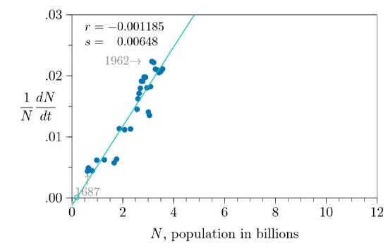
Figure \(\PageIndex{1}\) plots the two green columns of Table 6.1.1 through line 12—the mid-1960s—in blue dots, with a green line representing the average trend. A line like this can be drawn through the points in various ways—the simplest with a ruler and pen drawing what looks right. This one was done using a statistical “regression” program, with r the point at which the line intersects the vertical axis and s the line’s slope— its ∆y /∆x. The intrinsic growth rate r for modern, global human population is apparently negative and the slope s is unmistakably positive.

From the late 1600s to the mid 1960s, then, it’s clear that the birth rate per family was increasing as the population increased. Greater population was enhancing the population’s growth. Such growth is orthologistic, meaning that the human population has been heading for a singularity for many centuries. The singularity is not a modern phenomenon, and could conceivably have been known before the 20^th century.

The negative value of r, if it is real, means there is a human Allee point. If the population were to drop below the level of the intersection with the horizontal axis—in this projection, around two hundred million people—the human growth rate would be negative and human populations would decline. The Allee point demonstrates our reliance on a modern society; it suggests that we couldn’t survive with our modern systems at low population levels—although perhaps if we went back to hunter–gatherer lifestyles, this would change the growth curve. The Allee point thus indicates that there is a minimum human population we must sustain to avoid extinction. We depend on each other.