
4.2: Density-enhanced growth
- Page ID
- 25437

Darwin made unparalleled use of a model that failed, but how can the model be improved so that it does not fail?
Think of only three Black-Eyed Susan plants (Rudbeckia hirta) becoming established in Yellowstone National Park, one near the north-east entrance, one in the center, and a third near the south entrance—the plants thus separated by over 30 miles. How often would the same pollinator be able to visit two of the plants so the plants could reproduce? Rarely or never, because these pollinators travel limited distances. The plant’s growth rate will thus be 0. (In fact, it will be negative, since the three plants will eventually die.)
Suppose instead that 1000 of these plants were scattered about the park, making them about 2 miles apart. Occasionally a pollinator might happen by, though the chance of it visiting one of the other Black-Eyed Susans would be very low. Still, with 1000 plants in the area, the growth rate could be slightly positive.
Now consider 1,000,000 of those plants, making them about 100 meters apart. Pollination would now become relatively frequent. The growth rate of the population thus depends on the number of plants in the vicinity, meaning that this number must be part of the equation used to calculate the population growth rate.
We can use the equation introduced earlier to calculate this rate. First, put a parameter in place of the 1, like this.
\(\frac{1}{N}\, \frac{∆N}{∆t}\, =\,r\), where r formerly was 1
Then attach a term that recognizes the density of other members of the population, N.
\(\frac{1}{N}\, \frac{∆N}{∆t}\, =\,r\,+\,sN\),
Here r is related to the number of offspring each plant will produce if it is alone in the world or in the area, and s is the number of additional offspring it will produce for each additional plant that appears in its vicinity.
Suppose r = 0 and s = 1/20, just for illustration, and start with three plants, so N (0) = 3. That is
\(\frac{1}{N}\, \frac{∆N}{∆t}\, =\,0\,+\,0.05\,N\),
For watching the dynamics of this, multiply it out again
\(\frac{∆N}{∆t}\, =\,(0\,+\,0.05\,N)\,N\),
and convert the model to computer code, like this.
r=0; s=0.05; dt=1; t=0; N=3; print(N);
while(t<=14)
{ dN=(r+s*N)*N*dt; N=N+dN; t=t+dt; print(N); }
If you run this model in R (or other languages in which this code works, like C or AWK), you will see the numbers below.
3
3.45
4.045125
4.863277
6.045850
7.873465
10.97304
16.99341
31.43222
80.83145
407.5176
8,711.049
3,802,830
723,079,533,905
26,142,200,000,000,000,000,000
Graph these, and you will see the numbers expand past all bounds, vertically off the page.
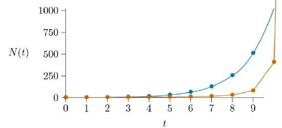
The blue line shows the unlimited bacterial growth (exponential growth) that helped lead Darwin to his idea of natural selection. The red line illustrates the new “density-enhanced growth” just being considered, where growth rate increases with density.
Because it approaches a line that is orthogonal to the line approached by the logistic model, described later, we call this an “orthologistic model.” It runs away to infinity so quickly that it essentially gets there in a finite amount of time. In physics and mathematics this situation is called a “singularity”—a place where the rules break down. To understand this, it is important to remember that all models are simplifications and therefore approximations, and apply in their specific range. The orthologistic model applies well at low densities, where greater densities mean greater growth. But a different model will take over when the densities get too high. In fact, if a population is following an orthologistic model, the model predicts that there will be some great change that will occur in the near future—before the time of the singularity.
In physics, models with singularities command special attention, for they can reveal previously unknown phenomena. Black holes are one example, while a more mundane one from physics is familiar to all. Consider a spinning coin with one point touching the table, spinning ever more rapidly as friction and gravity compel the angle between the coin and the table to shrink with time. It turns out that the physical equations that quite accurately model this spinning coin include a singularity—a place where the spinning of the coin becomes infinitely fast at a definite calculable time. Of course, the spinning cannot actually become infinitely fast. As the coin gets too close to the singularity—as its angle dips too near the table—it merely switches to a different model. That different model is a stationary coin. The exact nature of the transition between the spinning and stationary states is complex and debated, but the inevitability of the transition is not.
It is no different in ecology. Reasonable models leading to singularities are not to be discounted, but rather considered admissible where they apply. They arise inescapably in human population growth, considered in the next chapter.