
13.3: Stochastic modeling
- Page ID
- 25501

Program \(\PageIndex{1}\) simulates harvesting at the so-called maximal sustainable yield. It introduces small random fluctuations in the population—so small that they cannot be discerned in a graph. The slight stochasticity makes the program take a different trajectory each time it runs, with widely different time courses. Inevitably, however, the populations drift below the Allee point and rapidly collapse, as in the sample run of the program shown in Figure \(\PageIndex{1}\).
In the age of sailing, at the arrow marked "A", fishing was high-effort but low-impact and fisheries stayed approximately at their carrying capacity, \(K\). “Optimal harvesting” was introduced once mathematical ecology combined with diesel technology, and fisheries helped feed the growing human and domestic animal populations, with fish populations near “maximum sustainable yield,” as expected. But throughout the 20th century, as shown on either side of the arrow marked "B", fish populations continued to decline, and before 2015—at the arrow marked "C"—it becomes clear that something is seriously amiss.
# SIMULATE ONE YEAR
#
# This routine simulates a differential equation for optimal harvesting
# through one time unit, such as one year, taking very small time steps
# along the way.
#
# The ’runif’ function applies random noise to the population. Therefore it
# runs differently each time and the collapse can be rapid or delayed.
#
# ENTRY: ’N’ is the starting population for the species being simulated.
#        ’H’ is the harvesting intensity, 0 to 1.
#        ’K’ is the carrying capacity of the species in question.
#        ’r’ is the intrinsic growth rate.
#        ’dt’ is the duration of each small time step to be taken throughout
#           the year or other time unit.
#
# EXIT:  ’N’ is the estimated population at the end of the time unit.
SimulateOneYear = function(dt)
{ for(v in 1:(1/dt))                  # Advance the time step.
  { dN = (r+s*N)*N - H*r^2/(4*s)*dt;  # Compute the change.
    N=N+dN; }                         # Update the population value.
  if(N<=0) stop("Extinction");        # Make sure it is not extinct.
  assign("N",N, envir=.GlobalEnv); }  # Export the results.
r=1.75; s=-0.00175; N=1000; H=0; # Establish parameters.
for(t in 1850:2100)                   # Advance to the next year.
{ if(t>=1900) H=1;                    # Harvesting lightly until 1990.
  print(c(t,N));                      # Display intermediate results.
  N = (runif(1)*2-1)*10 + N;          # Apply stochasticity.
  SimulateOneYear(1/(365*24)); }      # Advance the year and repeat.
Program \(\PageIndex{1}\). This program simulates maximal harvesting with small fluctuations in the populations.
What happened? A collapse is part of the dynamics of this kind of harvesting. Inevitable stochasticity in harvest combines unfavorably with an unstable equilibrium in the prey population. In some runs it collapses in 80 years, in others it may take 300. The timing is not predictable; the main predictable property of the simulation is that ultimately the system will collapse.
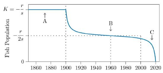
Figure \(\PageIndex{1}\). One sample run of Program 13.4, showing the collapse typical of such runs.