11.1: State Spaces

Closely related to “phase spaces” are “state spaces”. While phase spaces are typically used with continuous systems, described by differential equations, state spaces are used with discrete-time systems, described by difference equations. Here the natural system is approximated by jumps from one state to the next, as described in Chapter 7, rather than by smooth transitions. While the two kinds of spaces are similar, they differ in important ways.

Figure \(\PageIndex{1}\). A prairie ecosystem setting seed in fall colors— Bluebird Prairie, U.S. Upper Midwest. If not burned, grazed, or mowed, grasslands can leave a thick layer of litter that inhibits the next year’s growth.

Inspired by the complexities of ecology, and triggered in part by Robert May’s bombshell paper of 1976, an army of mathematicians worked during the last quarter of the twentieth century to understand these complexities, focusing on discrete-time systems and state spaces. One endlessly interesting state space is the delayed logistic equation (Aronson et al. 1982), an outgrowth of the discrete-time logistic equation described in Chapter 7.

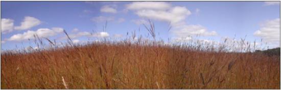
For a biological interpretation of the delayed logistic equation, let’s examine the example of live grassland biomass coupled with last year’s leaf litter. Biomass next year (N_t+1) is positively related to biomass this year (N_t), but negatively related to biomass from the previous year (N_t−1). The more biomass in the previous year, the more litter this year and the greater the inhibitory shading of next year’s growth. The simplest approximation here is that all biomass is converted to litter, a fixed portion of the litter decays each year, and inhibition from litter is linear. This is not perfectly realistic, but it has the essential properties for an example. Field data and models have recorded this kind of inhibition (Tilman and Wedin, Nature 1991).

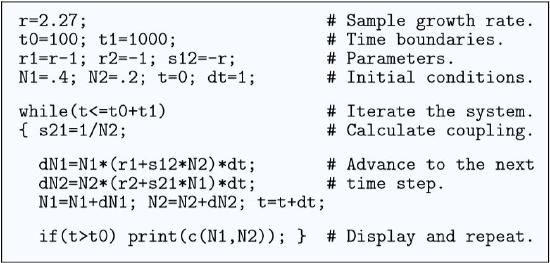
Program \(\PageIndex{1}\). A program to compute successive points in the state space of the delayed logistic equation.

The basic equation has N₁ as live biomass and N₂ as accumulated leaf litter. N₁ and N₂ are thus not two different species, but two different age classes of a single species.

\(N_1\,(t\,+\,1)\,=\,rN_1(t)\,(1\,-\,N_2(t))\)

\(N_2\,(t\,+\,1)\,=\,N_1\,(t)\,+\,pN_2\,(t)\)

The above is a common way to write difference equations, but subtracting N_i from each side, dividing by N_i , and making p = 0 for simplicity gives the standard form we have been using.

\(\frac{1}{N_1}\frac{∆N_1}{∆t}\,=\,(r\,-\,1)\,-\,rN_2\,=\,r_1\,+\,s_{1,2}N_2\)

\(\frac{1}{N_2}\frac{∆N_2}{∆t}\,=\,-1\,+\frac{1}{N_2}\,N_1\,=\,r_2\,+\,s_{2,1}N_1\)

Notice something new. One of the coefficients, s_2,1, is not a constant at all, but is the reciprocal of a dynamical variable. You will see this kind of thing again at the end of the predator–prey chapter, and in fact it is quite a normal result when blending functions (Chapter 18) to achieve a general Kolomogorov form. So the delayed logistic equation is as follows:

\(\frac{1}{N_1}\frac{∆N_1}{∆t}\,=\,r_1\,+\,s_{1,2}N_2\)

\(\frac{1}{N_2}\frac{∆N_2}{∆t}\,=\,r_2\,+\,s_{2,1}N_1\)

where r₁ = r−1, r₂ = −1, s_1,2 = −r, and s_2,1 = 1/N₁. Notice also that r_i with a subscript is different from r without a subscript.

Figure \(\PageIndex{2}\). Delayed logistic phase space with r =1.9, spiraling inward toward an equilibrium.

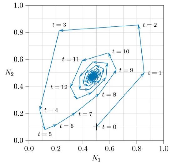
For small values of r, biomass and litter head to an equilibrium, as in the spiraling path of Figure \(\PageIndex{2}\). Here the system starts at the plus sign, at time t = 0, with living biomass N₁ =0.5 and litter biomass N₂ =0.1. The next year, at time t =1, living biomass increases to N₁ =0.85 and litter to N₂ = 0.5. The third year, t = 2, living biomass is inhibited slightly to N₁ = 0.81 and litter builds up to N₂ = 0.85. Next, under a heavy litter layer, biomass drops sharply to N₁ =0.22, and so forth about the cycle. The equilibrium is called an “attractor” because populations are pulled into it.

Figure \(\PageIndex{3}\). Delayed logistic phase space with r=2.03, spiraling toward a stable limit cycle, with the equilibrium point for r=1.9 shown as a dot.

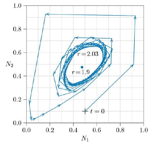
For larger values of r, the equilibrium loses its stability and the two biomass values, new growth and old litter, permanently oscillate around the state space, as in the spiraling path of Figure \(\PageIndex{3}\). The innermost path is an attractor called a “limit cycle.” Populations starting outside of it spiral inward, and populations starting inside of it spiral outward— except for populations balanced precariously exactly at the unstable equilibrium point itself.

Figure \(\PageIndex{4}\). Delayed logistic phase space with a stable equilibrium and three stable limit cycles for r = 1.9 to r = 2.27, as marked.

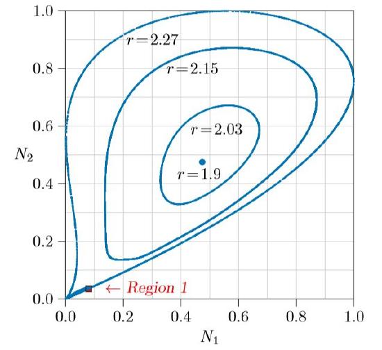
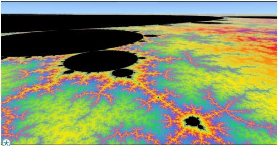
For still larger values of r, the system moves in and out of chaos in a way that itself seems chaotic. By r = 2.15 in Figure \(\PageIndex{4}\), the limit cycle is becoming slightly misshapen in its lower left. By r = 2.27 it has become wholly so, and something very strange has happened. A bulge has appeared between 0 and about 0.5 on the vertical axis, and that bulge has become entangled with the entire limit cycle, folded back on itself over and over again. What happens is shown by magnifying Region 1, inside the red square.

Figure \(\PageIndex{5}\) shows the red square of Figure \(\PageIndex{4}\) magnified 50 diameters. The tilted U-shaped curve is the first entanglement of the bulge, and the main part of the limit cycle is revealed to be not a curve, but two or perhaps more parallel curves. Successive images of that bulge, progressively elongated in one direction and compressed in the other, show this limit cycle to be infinitely complex. It is, in fact, not even a one-dimensional curve, but a “fractal,” this one being greater than one-dimensional but less than two-dimensional!

Figure \(\PageIndex{4}\) magnified 50 diameters.

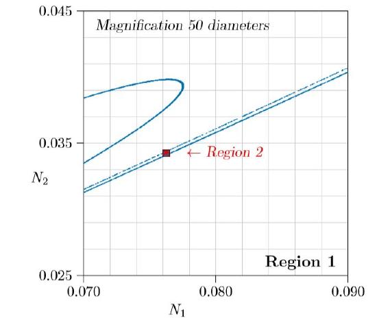
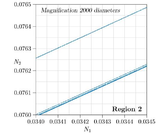
Figure \(\PageIndex{6}\) magnifies the red square of Figure \(\PageIndex{5}\), an additional 40 diameters, for a total of 2000 diameters. The upper line looks single, but the lower fatter line from Figure \(\PageIndex{5}\) is resolved into two lines, or maybe more. In fact, every one of these lines, magnified sufficiently, becomes multiple lines, revealing finer detail all the way to infinity! From place to place, pairs of lines fold together in U-shapes, forming endlessly deeper images of the original bulge. In the mathematical literature, this strange kind of attractor is, in fact, called a “strange attractor.”

Figure \(\PageIndex{5}\) magnified an additional 40 diameters.

Such strange population dynamics that occur in nature, with infinitely complex patterns, cannot arise in phase spaces of dynamical systems for one or two species flowing in continuous time, but can arise for three or more species in continuous time. And as covered in Chapter 7, they can arise for even a single species approximated in discrete time.

What we have illustrated in this chapter is perhaps the simplest ecological system with a strange attractor that can be visualized in a two-dimensional state space.

Figure \(\PageIndex{7}\). Landscape of the Mandelbrot set, which has been called the most complex object envisioned by the human mind. It is the division between two different behaviors in a particular two-dimensional dynamical system—an infinitely complex object that is less than 2-dimensional but greater than 1.9-dimensional. We display it here for your enjoyment—for wonder and for art.