10.3: Surface generating the flow

Think about shapes on which a marble could remain stationary, possibly balanced precariously, on a complicated two-dimensional surface in three-dimensional space, with peaks and valleys in their structure. Figure \(\PageIndex{1}\) shows seven possible configurations for remaining stationary.

Figure \(\PageIndex{1}\). Seven kinds of equilibria possible as part of surfaces defining two-species phase spaces.

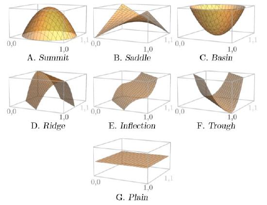
Configuration A is a summit, a high point with respect to its surroundings. It curves downward in every direction. It is therefore unstable—a marble perched on top can roll away in any direction.

Configuration C is the opposite, a basin. The surface curves upward in every direction. It is stable because a marble resting at the bottom rolls back from a disturbance in any direction.

Configuration B is like a combination of A and C. It is called a “saddle” for its once-ubiquitous shape (right). It curves upward in some directions and downward in others. A marble resting at its very center is unstable because it can roll away in many directions.

Configurations D, E, and F are related to A, B, and C, but are level in at least one direction. A “ridge,” Configuration D, has equilibria all along its very top. A marble balanced precariously there and nudged could conceivably move to a new equilibrium along the ridge, if the nudge were aligned with infinite exactitude; almost certainly, however, the marble would roll off. This configuration has an infinite number of equilibria—all along the ridge—but none of them are stable.

A “trough,” Configuration F, is the opposite of a ridge, with equilibria all along its lowest levels. A marble resting there and nudged will move to a new equilibrium position at the base of the trough. Again there are an infinite number of equilibria—all along the base—but none are stable because, pushed along the trough, the marble does not return to its previous location. The equilibria are neutrally stable, however, in the ecological view.

An “inflection,” Configuration E, is like a combination of D and F, changing slope and becoming level, but then resuming the same direction as before and not changing to the opposite slope. It too has a level line with an infinite number of equilibria, all unstable, with marbles rolling away from the slightest nudge in half of the possible directions.

Configuration G, a perfectly flat “plain,” is perhaps easiest to understand. A marble can rest anywhere, so every point on the flat surface is an equilibrium. But a marble will not return to its former position if nudged, so no equilibrium on the flat surface is stable. In ecology this situation is sometimes called “neutrally stable;” in mathematics it is called “unstable.”

With three-dimensional images and human cognitive power, it is possible to visualize a surface at a glance, such as in Figure 10.1.1, and judge the implications for populations growing according to equations that correspond to that surface. You can see at a glance if it is curving up everywhere or down everywhere, if it combines upward and downward directions, or if it has level spots. You can classify each equilibrium into the configurations of Figure \(\PageIndex{1}\). But how can that judgment be quantified, made automatic?

The method of eigenvectors and eigenvalues accomplishes this. Think of the prefix eigen- as meaning “proper,” as in “proper vector” or “proper value.” The idea will become clear shortly. The method of eigenvectors and eigenvalues was developed in stages over the course of more than two centuries by some of the best mathematical minds, and now we can apply it intact to ecology.

Figure 10.1.1, with the slope of the surface (its first derivative, dy/dx, middle) and changes in that slope (its second derivative, d ²y/dx², bottom)

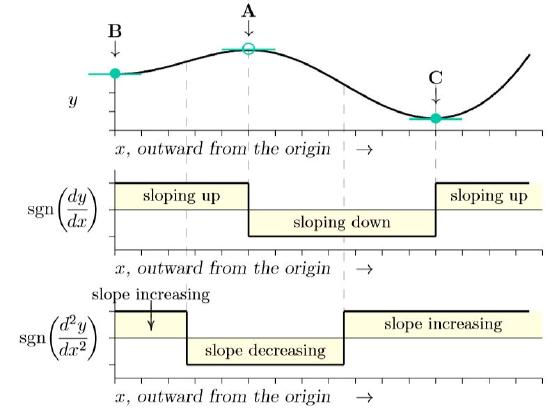
Think of a one-dimensional slice through the surface of Figure 10.1.1, successively passing through points B, A, C, and beyond. It would look like the top of Figure \(\PageIndex{2}\) As before, a marble balanced precisely at A would be unstable, ready to roll either toward B or C. The equilibrium points are level points where the slope is zero, as they are on the surface of Figure 10.1.1 From calculus, this is where the derivative is zero, where dy /dx = 0. Those slopes of zero are marked by green horizontal lines in the figure.

The middle graph of Figure \(\PageIndex{2}\) shows sign of the derivative, dy/dx, plus or minus. The sign function on the vertical axis, sgn(u ), is equal to zero if u is zero but is equal to plus or minus one if u is positive or negative, respectively. Whether an equilibrium is in a trough or at a summit is determined by how the slope is changing exactly at the equilibrium point. From calculus, that is the second derivative, \(\frac{d^2y}{dx^2}\), recording changes in the first derivative, dy/dx —just as the first derivative records changes in the surface itself.

The sign of the second derivative is shown in the bottom part of Figure \(\PageIndex{2}\). Wherever the slope is increasing at an equilibrium point—that is, changing from sloping down on the left to sloping up on the right—that is a basin. Wherever it is decreasing at an equilibrium point—changing from sloping up at the left to sloping down at the right—that is a summit. Whether an equilibrium point is stable or not can thus be determined mathematically merely from the sign of the second derivative of surface at that point!

This is easy if there is only one species, as in the models of earlier chapters, with only one direction to consider. But it becomes tricky when two or more species are interacting, for an infinite number of directions become available.

Figure \(\PageIndex{3}\) Partial derivatives, eigenvectors, and stability.

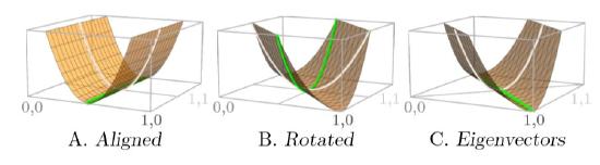
It might seem that a configuration will be a basin if the surface curves upward in both the x and y directions, as in Configuration C of Figure \(\PageIndex{1}\). But have a look at the three parts of Figure \(\PageIndex{3}\). Part A is a surface with a trough aligned with the axes.

Looking along the x-axis—which would be the N₁ axis showing the abundance of Species 1—the surface is curving up on both sides of its minimum (white curve). However, looking along the y -axis—the N₂ axis showing the abundance of Species 2—reveals that it is exactly level in that direction (green line), meaning the equilibrium is not stable.

But suppose the same surface is rotated 45 degrees, as in part B of the figure. The surface curves upward not only along the x -axis (white curve) but also along the y -axis (green curve). Yet the surface is the same. Contrary to what might have been expected, curving upward in both the x and y directions does not mean the configuration is a basin! Understanding the structure means looking in the proper directions along the surface, not simply along the axes.

This is what eigenvalues and eigenvectors do. They align with the “proper” axes for the surface, as illustrated in part C. No matter how twisted, skewed, or rescaled the surface is with respect to the axes, the eigenvectors line up with the “proper” axes of the surface, and the eigenvalues measure whether the slope is increasing or decreasing along those axes at an equilibrium.

Box \(\PageIndex{1}\) rules of eigenvalues for hill-climbing systems

1. If all eigenvalues are negative, the equilibrium is stable.
2. If any eigenvalue is positive, the equilibrium is unstable.
3. If some or all of the eigenvalues are zero and any remaining eigenvalues are negative, there is not enough information in the eigenvalues to know whether the equilibrium is stable or not. A deeper look at the system is needed.

In short, if all the eigenvalues are positive, the equilibrium is a basin, as in Figures 10.1.1C and \(\PageIndex{1}\)C. If all the eigenvalues are negative, the equilibrium is a summit, as in Figures 10.1.1A and \(\PageIndex{1}\)A. And if the eigenvalues are of mixed signs, or if some are zero, then we get one of the other configurations. (See Box \(\PageIndex{1}\))

he influence of gravity. Dynamical systems can do the opposite— they can climb to the highest level in the locality. For example, natural selection is commonly described as climbing “fitness peaks” on abstract “adaptive landscapes.” Of course, for mathematical surfaces rather than real mountain ranges, this is just a point of view. Whether a system climbs up or slides down depends arbitrarily on whether the mathematical surface is affixed with a plus or a minus sign in the equations.

Figure \(\PageIndex{2}\), an equilibrium in a hill-climbing system is stable if the slope is decreasing (negative sign) rather than increasing (positive sign). Because human intuition applies so well to marbles rolling off heights and settling into shallows, we have chosen to explain it intuitively that way first, but it is important to understand both ways.

It turns out that the proper axes at each equilibrium point—the eigenvectors—can be determined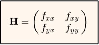 exactly from only four numbers, and how much the slope is increasing or decreasing at each equilibrium point— the eigenvalues—can be determined at the same time from the same four numbers. These are the four partial derivatives in what is called the “Hessian matrix” of the surface, or, equivalently in the “Jacobian matrix” of the population growth equations. An understanding of these matrices and their applications has developed in mathematics over the past two centuries.

By expending some effort and attention you can work the eigenvalues out mathematically with pencil and paper. However, you will likely employ computers to evaluate the eigenvalues of ecological systems. This can be done with abstract symbols in computer packages such as Mathematica or Maxima, or numerically in programming languages such as R. For standard two-species systems, we have worked out all equilibria and their corresponding eigenvalues. These are recorded in Table \(\PageIndex{1}\) in mathematical notation and in Program \(\PageIndex{1}\) as code, and identify the equilibria and stability for all predation, mutualism, and competition systems represented by the two-species formulae, which is copied into the table for reference.

Table \(\PageIndex{1}\). Two-species formulae

Location	Equilibrium	Eigenvalues
Origin (Both species extinct)	(0,0)	\((\,r_1,\,r_2)\)
Horizontal axis (Species 1 at K1)	\(-\frac{r_1}{s_{1,1}}\,\,0\)	\(-r_1,\,\frac{q}{s_{1,1}}\,)\)
Vertical axis (Species 2 at K2)	\(0,\,-\frac{r_2}{s_{2,2}}\)	\(-r_2\,\frac{p}{s_{2,2}}\)
Interior (Coexistence)	\(\frac{p}{a}\,,\,\frac{q}{a}\)	\(\frac{-b\pm\sqrt{b^2-4ac}}{2a}\)

with

a = s_1,2 s_2,1 − s_1,1s_2,2

b = r₁ s_2,2 (s_2,1 −s_1,1) + r₂ s_1,1 (s_1,2 −s_2,2)

c = −pq

p = r₁ s_2,2 −r₂ s_1,2

q = r₂ s_1,1 −r₁ s_2,1

in the ecological equations for two interacting species,

\(\frac{1}{N_1}\,\frac{dN_1}{dt}\,=\,r_1\,+\,s_{1,1}N_1\,+\,s_{1,2}N_2\)

\(\frac{1}{N_2}\,\frac{dN_2}{dt}\,=\,r_2\,+\,s_{2,2}N_1\,+\,s_{2,1}N_1\)

where

N₁, N₂ are population abundances of Species 1 and 2

r₁, r₂ are intrinsic growth rates

s_1,1, s_2,2 measure species effects on themselves

s_1,2, s_2,1 measure effects between species

p = r1*s22 -r2*s12; # Compute useful sub

q = r2*s11 -r1*s21; # formulae.

a = s12*s21 -s11*s22;

b = r1*s22*(s21-s11) +r2*s11*(s12-s22);

c = -p*q; # Compute the equilibria.

x00=0; y00=0; # (at the origin)

x10=-r1/s11; y10=0; # (on the x-axis)

x01=0; y01=-r2/s22; # (on the y-axis)

x11=p/a; y11=q/a; # (at the interior)
v00= r1; w00=r2; # Compute the corresponding

v10=-r1; w10=q/s11; # four pairs of eigenvalues

v01=-r2; w01=p/s22; # (real part only).

v11=(-b-Sqrt(b^2-4*a*c))/(2*a);

w11=(-b+Sqrt(b^2-4*a*c))/(2*a);

Program \(\PageIndex{1}\). The code equivalent to Table \(\PageIndex{1}\), for use in computer programs. Sqrt(w) is a specially written function that returns 0 if w is negative (returns the real part of the complex number 0 +\(\sqrt{w}\,i\)).

The formulae in Table \(\PageIndex{1}\) work for any two-species RSN model—that is, any model of the form \(\frac{1}{N_i}\frac{dN_i}{dt}\,=\,r_1\,+\,s_{i,i}N_i\,+\,s_{i,j}N_j\) with constant coefficients—but formulae for other models must be derived separately, from a software package, or following methods for Jacobian matrices.

box \(\PageIndex{2}\) parameters for a sample Competitive system

\(r_1\,=\,1.2\)	\(r_2\,=\,0.8\)	Intrinisic growth rate
\(s_{1,1}\,=\,-1\)	\(s_{2,2}\,=\,-1\)	Self-limiting terms
\(s_{1,2}\,=\,-1.2\)	\(s_{2,1}\,=\,-0.5\)	Cross-limiting terms