27.7: Modeling Population and Allele Frequencies

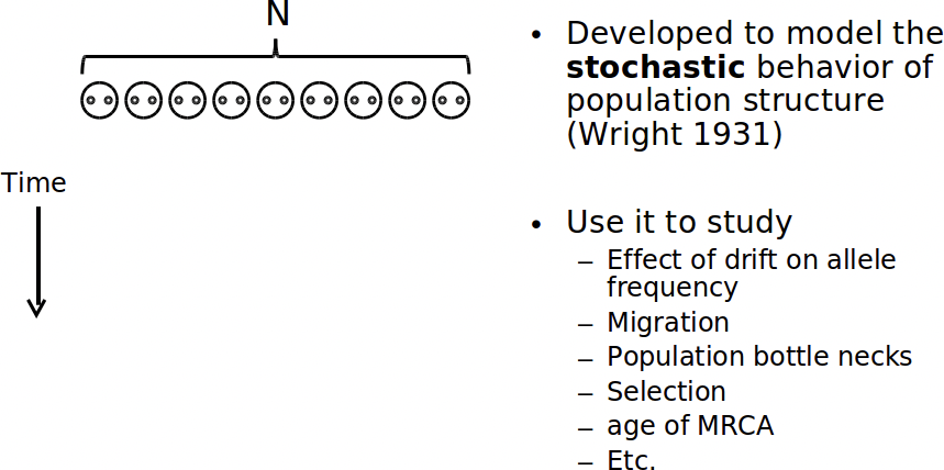
With the advent of next-gen sequencing, it is becoming economical to sequence the genomes of many individuals within a population. In order to make sense of how alleles spread through a population, it’s helpful to have a model to compare data against. The Wright-Fisher reproduction model has filled this role for the past 70 years.

The Wright-Fisher Model

Like HMMs, Wright-Fisher is a Markov process: at each step, the system randomly progresses, and the current state of the system depends only on the previous state. In this case, state transitions represent reproduction. By modeling the transmission of chromosomes to offspring, we can study genetic drift.

The model makes a number of simplifying assumptions:

1. Population size, N, is constant at each generation.
2. Only members of the same generation reproduce (no overlap).

3. Reproduction occurs at random.
4. The gene being modeled only has 2 alleles.
5. Genes undergo neutral selection.

Note that Wright-Fisher is not an appropriate choice if you’re trying to model the change in frequency of a gene that is positively or negatively selected for. If we use Wright-Fisher to model the chromosomes of diploid individuals, the population size of the model becomes 2N.

Figure 27.17: The Wright-Fisher model

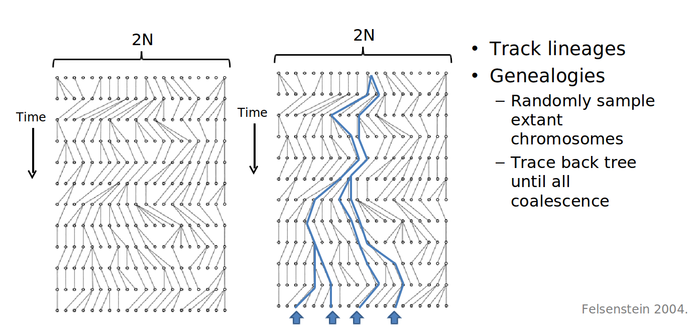
In English, here’s how Wright-Fisher works:

At every generation, for each child, we randomly select from the parents (with replaccement). The allele of the child becomes that of the randomly selected parent.

We repeat this process for many generation, with the children serving as the new parents, ignoring the ordering of chromosomes.

It really is that simple. To determine the probability of k copies of an allele existing in the child generation when it had a frequency of p in the parent generation, we can use this formula:

\[\left(\begin{array}{c}
2 N \\
k
\end{array}\right) p^{k} q^{2 N-k}\]

Here, q = (1-p). It is the frequency of non-p alleles in the parent generation.

Sinauer Associates, Inc. All rights reserved. This content is excluded from our Creative

Commons license. For more information, see http://ocw.mit.edu/help/faq-fair-use.

Figure 27.18: Many iterations of Wright-Fisher yielding a lineage tree

Now we can begin to explore such questions as: how probable is it and how many generations is it expected to take for a given allele to become fixed, meaning the allele is present in every member of the population?

The expected time (in generations) for fixation, given the assumptions made by Wright-Fisher, is proportionate to 4N_E, where NE is the effective population size.

Again, it’s important to keep in mind the limitations of this model and ask if it actually makes sense for the system you’re trying to represent. Consider how you could tweak the proposed model to account for a selection coecient ranging between -1 (lethal negative selection) and 1 (strong positive selection).

The Coalescent Model

The problem with the Wright-Fisher model is that it assumes you know the allele frequencies of the ancentral generation. When dealing with the genomes of present species, these quantities are unknown. The Coalescent Model solves this conundrum by thinking retrospectively. That is to say: we start with the alleles of the current generation, and work our way backwards in time. The basic Coalescence Model makes the same assumptions as Wright-Fisher. At each generation, we ask: what is the probability of the two identical alleles coalescing, or sharing a parent, in the previous generation.

We can pose the probability of a coalescence event occuring in the previous generation as the probability of coalescence not occuring in any of the t-1 generations prior to the last one, times the probability of it occuring in the previous (the t-th) generation. This is equivalent to the expression:

\[P_{c}(t)=\left(1-\frac{1}{2 N_{e}}\right)^{t-1}\left(\frac{1}{2 N_{e}}\right)\]

Where N_e is the effective population size.

Figure 27.19: The coalescent model.

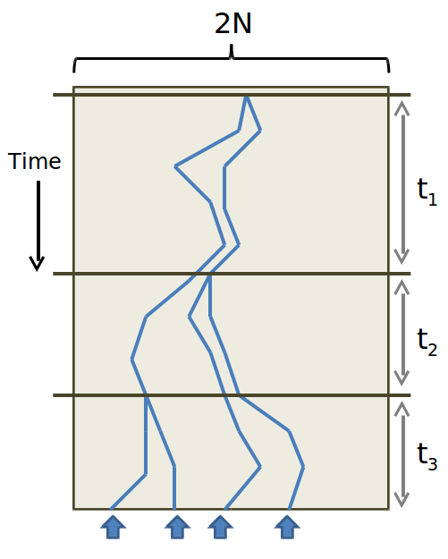
By approximating this geometric distribution as an exponential one: \(P_{c}(t)=\frac{1}{2 N_{e}} e^{-\left(\frac{t-1}{2 N_{e}}\right)}\), we can determine the expected number of generations back until coalescence, which turns out to be 2Ne, with a standard deviation of 2N_e.

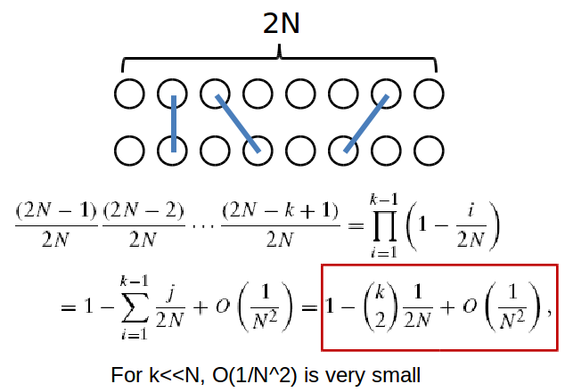
To ask about the coalescence of multiple lineages at a given generation, we must, as in Wright-Fisher, use a binomial distribution. The probability of k lineages coalescing for the first time at generation t is:

\[P\left(T_{k}=t\right)=\left(1-\left(\begin{array}{l}
k \\
2
\end{array}\right) \frac{1}{2 N}\right)^{t-1}\left(\begin{array}{l}
k \\
2
\end{array}\right) \frac{1}{2 N}\]

And again, this can be approximated with an exponential distribution for sufficiently large k. The individual at which two lineages converge is referred to as the Most Recent Common Ancestor. By continually moving backwards until all ancestors coalesce, we end up with a new kind of tree! And by comparing the tree resulting from coalescence with a gene tree we’ve constructed, discrepancies between the two may signal that certain assumptions of the Coalescent Model have been violated. Namely, selection may be occuring.

Figure 28.20: Geometric probability distribution for coalescent events in k lineages.

The Multispecies Coalescent Model

Figure 27.21: Multispecies Coalescent Model.

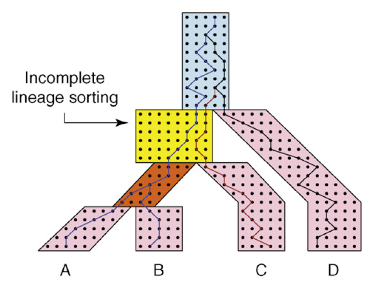
Courtesy of Elsevier, Incorporate. Used with permission.

Source: Degnan, James H., and Noah A. Rosenberg. "Gene Tree Discordance, Phylogenetic

Inference and the Multispecies Coalescent." Trends in Ecology & Evolution 24, no. 6 (2009): 332-40.

We can take this idea once step further and track coalescence events across multiple species. Here, each genome of an individual species is treated as a lineage.

Note that there is a lag time between the separation of two populations and the time at which two gene lineages coalesce into a common ancestor. Also note how the rate of coalescence slows down as N gets bigger and for short branches.

In the image above, deep coalescence is depicted in light blue for three lineages. The species and gene trees here are incongruent since C and D are sisters in gene tree but not the species tree.

There is a \(\frac{2}{3}\) chance that incongruence will occur because once we get to the light blue section, Wright- Fisher is memoryless and there is only \(\frac{1}{3}\) chance that it will be congruent. The effect of incongruence is called Incomplete Lineage Sorting. By measuring the frequency at which ILS occurs, we gain insight into unusually large populations or unsually short branch lengths within the species tree.

You can build a maximum parsimony species tree based on the notion of minimizing the number of ILS events rather than minimizing implied duplication/loss events as covered previously. It is even possible to combine these two methods to, ideally, create a phylogeny that is more accurate than either of them would be individually.