27.5: Inferring Orthologs/Paralogs, Gene Duplication and Loss

There are two commonly used trees, Species tree and Gene tree. This section explains how these trees can be used and how to fit a gene tree inside a species tree (reconciliation).

Species Tree

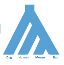
Species trees that show how different species evolved from one another. These trees are created using morphological characters, fossil evidence, etc. The leaves of each tree are labeled as species and the rest of the tree shows how these species are related. An example of a species tree is shown in Figure 27.1. Note: in lecture it is mentioned that a species can be thought of as a ”bag of genes”, that is to say the group of common genes among members of a species.

Gene Tree

Figure 27.1: Species Tree

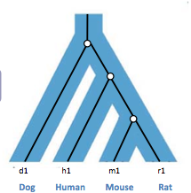
Gene trees are trees that look at specific genes in different species. The leaves of gene trees are labeled with gene sequences or gene ids associated with specific sequences. Figure 27.2 shows an example of a gene tree that has 4 genes (leaves). The sequences associated with each gene are presented on the right side of Figure 27.2.

Figure 27.2: Gene Tree

Gene Family Evolution

Gene trees evolve inside a species tree. An example of a gene tree contained in a species tree is shown in Figure 27.3 below.

Figure 27.3: Gene Tree Inside a Species Tree

The next sub section explains how we can fit gene trees inside a species trees using Reconciliation.

Reconciliation

Reconciliation is an algorithm that helps compare gene trees to genome trees by fitting a gene tree fits inside a species tree. This is done by by mapping the vertices in the gene tree to vertices in the species tree. This sub section will focus on Reconciliation, related definitions, algorithms (Maximum Parsimony Reconciliation and SPIDIR) and examples.

Definitions

Two genes are orthologs if their most recent common ancestor (MRCA) is a speciation (splitting into different species).
Paralogs are genes whose MRCA is a duplication.
Figure 27.4 below illustrates how these types of genes can be represented in a gene tree. The tree below has 4 speciation nodes, one duplication and one loss.

Figure 27.4: Gene Family Evolution: Gene Trees and Species Trees

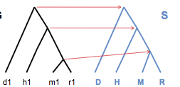
A mapping diagram is a diagram that shows the node mapping from the gene tree to the species tree. Figure 27.5 shows an example of a mapping diagram.

Figure 27.5: Mapping Diagram

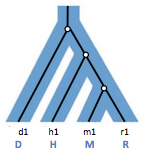
A nesting diagram shows how the gene tree can be nested inside the species tree. For every mapping diagram there is a nesting diagram. Figure 27.6 shows an example of a possible nesting diagram for the mapping diagram in Figure 27.5.

Figure 27.6: Nesting Diagram

Maximum Parsimony Reconciliation (MPR) Algorithm

MPR is an algorithm that fits a gene tree into a species tree while minimizing the number of duplications and deletions.

Figure 27.7: Maximum Parsimony Reconciliation (MPR)

Given a gene tree and a species tree, the algorithm finds the reconciliation that minimizes the number of duplications and deletions. Figure 27.7 above shows an example of a possible mapping from a gene tree to a species tree. Figure 27.8 presents the pseudocode for the MPR algorithm. The base case involves matching the leaves of the gene tree to the leaves of the species tree; the algorithm then progresses up the vertices of the gene tree, drawing a relationship between the MRCA of all leaves within a given vertex’s sub-tree and the corresponding MRCA vertex in the species tree. In the pseudocode, I(G) represents the species tree and L(G) represents the gene tree.

Figure 27.8: Maximum Parsimony Reconciliation Recursive Algorithm

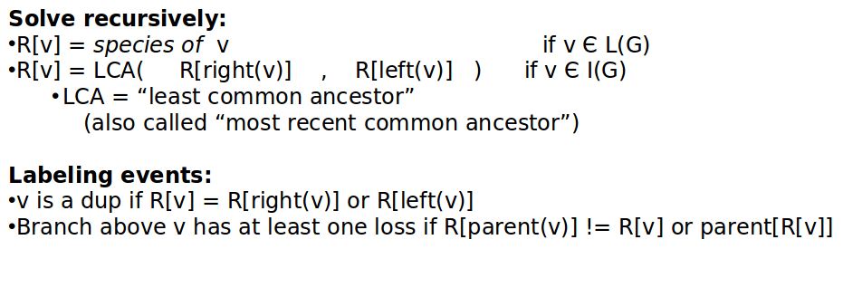
We map the arrows low as possible, since lower mapping usually results in fewer events. However, we cannot map too low. Mapping too low means that we’re violating the constraint that the MRCA of a given node is at least as high as the MRCA of its children. We map as low as we can without violating the descendent- ancestor relationships. The algorithm goes recursively from bottom up, starting from the leaves. Since we sample genes from known species to build the gene tree, there’s a direct mapping between the leaves of the gene tree and the leaves of the species tree. To map the ancestors, for each node (going recursively up the tree) we look at the right child and left child and take the least common ancestor (LCA) of the species that they map to. If a node maps to its right or left child, we know there is a duplication. An expected branch that does not exist indicates a loss.

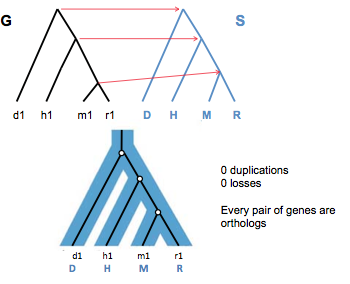
Reconciliation Examples

Figure 27.9: Reconciliation Example 1, simple mapping case

Figure 27.10: Reconciliation Example 2, parsimonious reconciliation for complex case

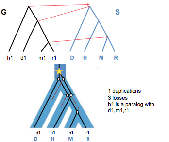
In Figure 27.10, we see a parsimonious (minimum number of losses and duplications) reconciliation for a case in which nodes from the gene tree cannot be mapped straight across. This is a result of the swapped locations of h1 and d1 in the gene tree; the least common ancestor for d1, m1, and r1 is now the root vertex of the species tree.

Figure 28.11: Reconciliation Example 3, non parsimonious reconciliation for complex case

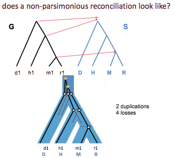
Figure 27.11 shows a non-parsimonious reconciliation . The parsimonious mapping for the same trees is shown in Figure 27.9.

Figure 27.12: Reconciliation Example 4, invalid Reconciliation

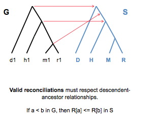
Figure 27.12 shows an invalid reconciliation. This reconciliation is invalid since it does not respect descendent- ancestor relationships. In order for this reconciliation to be possible, the descendent would have to travel back in time and be created before its ancestor. Clearly, such a scenario would be impossible. A valid reconciliation must satisfy the following: If a < b in G, then R[a] \(\leq\) R[b] in S.

Interpreting Reconciliation Examples

Gene trees, when reconciled with species trees, offer significant insight into evolutionary events (namely duplications and losses). Duplications describe the same gene being found at a separate loci - m2 or r2, in this situation - and is a major mechanism for creating new genes and functions. These evolutionary consequences fall into three categories: nonfunctionalization, neofunctionalization and subfunctionalization. Nonfunctionalization is quite common and causes one of the copies, unsurprisingly, to simply not function. Neofunctionalization is when one of the copies develops an entirely new function. Subfunctionalization is when the copies retain different parts (dividing up the labor, in a way), and together, perform the same function.

In Figure 4, we see that a duplication event occurred before the divergence of mice and rats as species. This is why we see similar genes at both m1 and m2, which represent two separate loci. d2 and h2 are not included in the graph because at the gene being considered is not present at those loci (since no duplication event occurred), whereas it is at both m2 and r2.

If the duplication event were to have occurred one level higher in Figure 4, without seeing a corresponding h2 in the gene tree, this would imply a loss within the h branch of the species tree.