21.6: Network clustering, Bibliography

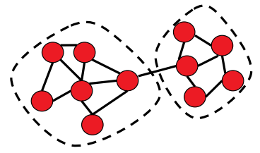
An important problem in network analysis is to be able to cluster or modularize the network in order to identify subgraphs that are densely connected (see e.g., figure 21.6a). In the context of gene interaction networks, these clusters could correspond to genes that are involved in similar functions and that are co- regulated.

There are several known algorithms to achieve this task. These algorithms are usually called graph partitioning algorithms since they partition the graph into separate modules. Some of the well-known algorithms include:

• Markov clustering algorithm [5]: The Markov Clustering Algorithm (MCL) works by doing a random walk in the graph and looking at the steady-state distribution of this walk. This steady-state distribution allows to cluster the graph into densely connected subgraphs.
• Girvan-Newman algorithm [2]: The Girvan-Newman algorithm uses the number of shortest paths going through a node to compute the essentiality of an edge which can then be used to cluster the network.
• Spectral partitioning algorithm

In this section we will look in detail at the spectral partitioning algorithm. We refer the reader to the references [2, 5] for a description of the other algorithms.

The spectral partitioning algorithm relies on a certain way of representing a network using a matrix. Before presenting the algorithm we will thus review how to represent a network using a matrix, and how to extract information about the network using matrix operations.

source unknown. All rights reserved. This content is

excluded from our Creative Commons license. For more

information, see http://ocw.mit.edu/help/faq-fair-use/.

(a) A partition of a network into two groups.

(b) A simple network on 3 nodes. The adjacency

matrix of this graph is given in equation (21.1) .

Figure 21.6

Algebraic view to networks

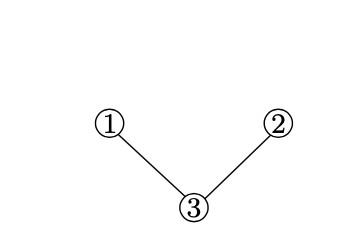
Adjacency matrix One way to represent a network is using the so-called adjacency matrix. The adjacency matrix of a network with n nodes is an n \(\times\) n matrix A where A_i,j is equal to one if there is an edge between nodes i and j, and 0 otherwise. For example, the adjacency matrix of the graph represented in figure 21.6b is given by:

\[A=\left[\begin{array}{lll}
0 & 0 & 1 \\
0 & 0 & 1 \\
1 & 1 & 0
\end{array}\right] \nonumber \]

If the network is weighted (i.e., if the edges of the network each have an associated weight), the definition of the adjacency matrix is modified so that Ai,j holds the weight of the edge between i and j if the edge exists, and zero otherwise.

Laplacian matrix For the clustering algorithm that we will present later in this section, we will need to count the number of edges between the two different groups in a partitioning of the network. For example, in Figure 21.6a, the number of edges between the two groups is 1. The Laplacian matrix which we will introduce now comes in handy to represent this quantity algebraically. The Laplacian matrix L of a network on n nodes is a n \(\times\) n matrix L that is very similar to the adjacency matrix A except for sign changes and for the diagonal elements. Whereas the diagonal elements of the adjacency matrix are always equal to zero (since we do not have self-loops), the diagonal elements of the Laplacian matrix hold the degree of each node (where the degree of a node is defined as the number of edges incident to it). Also the off-diagonal elements of the Laplacian matrix are set to be 1 in the presence of an edge, and zero otherwise. In other words, we have:

\[L_{i, j}=\left\{\begin{array}{ll}
\operatorname{degree}(i) & \text { if } i=j \\
-1 & \text { if } i \neq j \text { and there is an edge between } i \text { and } j \\
0 & \text { if } i \neq j \text { and there is no edge between } i \text { and } j
\end{array}\right. \nonumber \]

For example the Laplacian matrix of the graph of figure 21.6b is given by (we emphasized the diagonal elements in bold):

\[L=\left[\begin{array}{ccc}
1 & 0 & -1 \\
0 & 1 & -1 \\
-1 & -1 & 2
\end{array}\right] \nonumber \]

Some properties of the Laplacian matrix The Laplacian matrix of any network enjoys some nice properties that will be important later when we look at the clustering algorithm. We briefly review these here.

The Laplacian matrix L is always symmetric, i.e., Li,j = Lj,i for any i,j. An important consequence of this observation is that all the eigenvalues of L are real (i.e., they have no complex imaginary part). In fact one can even show that the eigenvalues of L are all nonnegative8 The final property that we mention about L is that all the rows and columns of L sum to zero (this is easy to verify using the definition of L). This means that the smallest eigenvalue of L is always equal to zero, and the corresponding eigenvector is s = (1,1,...,1).

Counting the number of edges between groups using the Laplacian matrix Using the Laplacian matrix we can now easily count the number of edges that separate two disjoint parts of the graph using simple matrix operations. Indeed, assume that we partitioned our graph into two groups, and that we define a vector s of size n which tells us which group each node i belongs to:

\[s_{i}=\left\{\begin{array}{ll}
1 & \text { if node } i \text { is in group } 1 \\
-1 & \text { if node } i \text { is in group } 2
\end{array}\right. \nonumber \]

Then one can easily show that the total number of edges between group 1 and group 2 is given by the quantity \(\frac{1}{4} s^{T}\) Ls where L is the Laplacian of the network.

To see why this is case, let us first compute the matrix-vector product Ls. In particular let us fix a node i say in group 1 (i.e., si = +1) and let us look at the i’th component of the matrix-vector product Ls. By definition of the matrix-vector product we have:

\[(L s)_{i}=\sum_{j=1}^{n} L_{i, j} s_{j} \nonumber \]

We can decompose this sum into three summands as follows:

\[(L s)_{i}=\sum_{j=1}^{n} L_{i, j} s_{j}=L_{i, i} s_{i}+\sum_{j \text { in group } 1} L_{i, j} s_{j}+\sum_{j \text { in group } 2} L_{i, j} s_{j} \nonumber \]

Using the definition of the Laplacian matrix we easily see that the first term corresponds to the degree of i, i.e., the number of edges incident to i; the second term is equal to the negative of the number of edges connecting i to some other node in group 1, and the third term is equal to the number of edges connecting i to some node ingroup 2. Hence we have:

(Ls)_i = degree(i) (# edges from i to group 1) + (# edges from i to group 2)

Now since any edge from i must either go to group 1 or to group 2 we have:

degree(i) = (# edges from i to group 1) + (# edges from i to group 2).

Thus combining the two equations above we get:

(Ls)_i = 2 ⇥ (# edges from i to group 2).
Now to get the total number of edges between group 1 and group 2, we simply sum the quantity above

over all nodes i in group 1:
\[\text { (# edges between group 1 and group 2) }=\frac{1}{2} \sum_{i \text { in group } 1}(L s)_{i} \nonumber\]

We can also look at nodes in group 2 to compute the same quantity and we have:

\[\text { (# edges between group 1 and group 2) }=-\frac{1}{2} \sum_{i \text { in group 2 }}(L s)_{i} \nonumber \]

Now averaging the two equations above we get the desired result:

\[\begin{aligned}
&\text { (# edges between group 1 and group 2) }=\frac{1}{4} \sum_{i \text { in group 1 }}(L s)_{i}-\frac{1}{4} \sum_{i \text { in group 2 }}(L s)_{i}\\
&\begin{array}{l}
=\frac{1}{4} \sum_{i} s_{i}(L s)_{i} \\
=\frac{1}{4} s^{T} L s
\end{array}
\end{aligned} \nonumber \]

where sT is the row vector obtained by transposing the column vector s.

The spectral clustering algorithm

We will now see how the linear algebra view of networks given in the previous section can be used to produce a “good” partitioning of the graph. In any good partitioning of a graph the number of edges between the two groups must be relatively small compared to the number of edges within each group. Thus one way of addressing the problem is to look for a partition so that the number of edges between the two groups is minimal. Using the tools introduced in the previous section, this problem is thus equivalent to finding a vector\(s \in\{-1,+1\}^{n}\) taking only values 1 or +1 such that \(\frac{1}{4} s^{T}\) Ls is minimal, where L is the Laplacian matrix of the graph. In other words, we want to solve the minimization problem:

\(\operatorname{minimize}_{s \in\{-1,+1\}^{n}} \frac{1}{4} s^{T} L s \nonumber \)

If s^* is the optimal solution, then the optimal partioning is to assign node i to group 1 if s_i = +1 or else to group 2.

This formulation seems to make sense but there is a small glitch unfortunately: the solution to this problem will always end up being s = (+1,...,+1) which corresponds to putting all the nodes of the network in group 1, and no node in group 2! The number of edges between group 1 and group 2 is then simply zero and is indeed minimal!

To obtain a meaningful partition we thus have to consider partitions of the graph that are nontrivial. Recall that the Laplacian matrix L is always symmetric, and thus it admits an eigendecomposition:

\[L=U \Sigma U^{T}=\sum_{i=1}^{n} \lambda_{i} u_{i} u_{i}^{T}\nonumber\]

where \(\sigma\) is a diagonal matrix holding the nonnegative eigen values \(\lambda_{1}, \ldots, \lambda_{n}\) of L and U is the matrix of eigenvectors and it satisfies U^T=U-¹.

The cost of a partitioning \(s \in\{-1,+1\}^{n}\) is given by

\[\frac{1}{4} s^{T} L s=\frac{1}{4} s^{T} U \Sigma U^{T} s=\frac{1}{4} \sum_{i=1}^{n} \lambda_{i} \alpha_{i}^{2}\nonumber\]

where \(\alpha=U^{T}s\) give the decomposition of s as a linear combination of the eigenvectors of L: \(s=\sum_{i=1}^{n} \alpha_{i} u_{i}\).

source unknown. All rights reserved. This content is excluded from our Creative

Commons license. For more information, see http://ocw.mit.edu/help/faq-fair-use/.

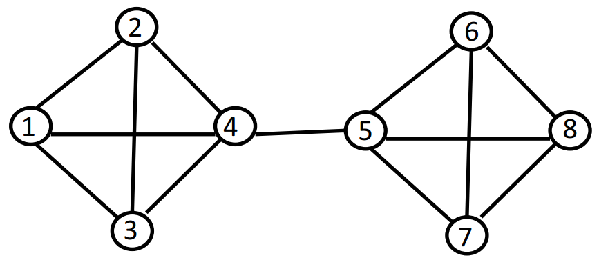
Figure 21.7: A network with 8 nodes

Recall also that \(0=\lambda_{1} \leq \lambda_{2} \leq \cdots \leq \lambda_{n}\). Thus one way to make the quantity above as small as possible (without picking the trivial partitioning) is to concentrate all the weight on \(\lambda_{2}\) which is the smallest nonzero eigenvalue of L. To achieve this we simply pick s so that \(\alpha_{2}\) =1 and \(\alpha_{k}\) = 0 for all k \(\neq\) 2. In other words, this corresponds to taking s to be equal to u₂ the second eigenvector of L. Since in general the eigenvector u₂ is not integer-valued (i.e., the components of u₂ can be different than 1 or +1), we have to convert first the vector u₂ into a vector of +1’s or 1’s. A simple way of doing this is just to look at the signs of the components of u₂ instead of the values themselves. Our partition is thus given by:

\[s=\operatorname{sign}\left(u_{2}\right)=\left\{\begin{array}{ll}
1 & \text { if }\left(u_{2}\right)_{i} \geq 0 \\
-1 & \text { if }\left(u_{2}\right)_{i}<0
\end{array}\right.\nonumber\]

To recap, the spectral clustering algorithm works as follows:

Spectral partitioning algorithm

• Input: a network
• Output: a partitioning of the network where each node is assigned either to group 1 or group

  2 so that the number of edges between the two groups is small

1. Compute the Laplacian matrix L of the graph given by:

   \[L_{i, j}=\left\{\begin{array}{ll}
   \operatorname{degree}(i) & \text { if } i=j \\
   -1 & \text { if } i \neq j \text { and there is an edge between } i \text { and } j \\
   0 & \text { if } i \neq j \text { and there is no edge between } i \text { and } j
   \end{array}\right.\nonumber\]

2. Compute the eigenvector u₂ for the second smallest eigenvalue of L.
3. Output the following partition: Assign node i to group 1 if (u₂)_i \(\geq\)0, otherwise assign node i to group 2.

We next give an example where we apply the spectral clustering algorithm to a network with 8 nodes.

Example We illustrate here the partitioning algorithm described above on a simple network of 8 nodes given in figure 21.7. The adjacency matrix and the Laplacian matrix of this graph are given below:

\[A=\left[\begin{array}{llllllll}
0 & 1 & 1 & 1 & 0 & 0 & 0 & 0 \\
1 & 0 & 1 & 1 & 0 & 0 & 0 & 0 \\
1 & 1 & 0 & 1 & 0 & 0 & 0 & 0 \\
1 & 1 & 1 & 0 & 1 & 0 & 0 & 0 \\
0 & 0 & 0 & 1 & 0 & 1 & 1 & 1 \\
0 & 0 & 0 & 0 & 1 & 0 & 1 & 1 \\
0 & 0 & 0 & 0 & 1 & 1 & 0 & 1 \\
0 & 0 & 0 & 0 & 1 & 1 & 1 & 0
\end{array}\right] \quad L=\left[\begin{array}{rrrrrr}
3 & -1 & -1 & -1 & 0 & 0 & 0 & 0 \\
-1 & 3 & -1 & -1 & 0 & 0 & 0 & 0 \\
-1 & -1 & 3 & -1 & 0 & 0 & 0 & 0 \\
-1 & -1 & -1 & 4 & -1 & 0 & 0 & 0 \\
0 & 0 & 0 & -1 & 4 & -1 & -1 & -1 \\
0 & 0 & 0 & 0 & -1 & 3 & -1 & -1 \\
0 & 0 & 0 & 0 & -1 & -1 & 3 & -1 \\
0 & 0 & 0 & 0 & -1 & -1 & -1 & 3
\end{array}\right] \nonumber \]
Using the eig command of Matlab we can compute the eigendecomposition \(L=U \Sigma U^{T}\) of the Laplacian matrix and we obtain:

\[U=\left[\begin{array}{rrrrrrr}
0.3536 & -0.3825 & 0.2714 & -0.1628 & -0.7783 & 0.0495 & -0.0064 & -0.1426 \\
0.3536 & -0.3825 & 0.5580 & -0.1628 & 0.6066 & 0.0495 & -0.0064 & -0.1426 \\
0.3536 & -0.3825 & -0.4495 & 0.6251 & 0.0930 & 0.0495 & -0.3231 & -0.1426 \\
0.3536 & -0.2470 & -0.3799 & -0.2995 & 0.0786 & -0.1485 & 0.3358 & 0.6626 \\
0.3536 & \mathbf{0 . 2 4 7 0} & -0.3799 & -0.2995 & 0.0786 & -0.1485 & 0.3358 & -0.6626 \\
0.3536 & \mathbf{0 . 3 8 2 5} & 0.3514 & 0.5572 & -0.0727 & -0.3466 & 0.3860 & 0.1426 \\
0.3536 & \mathbf{0 . 3 8 2 5} & 0.0284 & -0.2577 & -0.0059 & -0.3466 & -0.7218 & 0.1426 \\
0.3536 & \mathbf{0 . 3 8 2 5} & 0.0000 & 0.0000 & 0.0000 & 0.8416 & -0.0000 & 0.1426
\end{array}\right]\nonumber\]

\[\Sigma=\left[\begin{array}{llllllll}
0 & 0 & 0 & 0 & 0 & 0 & 0 & 0 \\
0 & 0.3542 & 0 & 0 & 0 & 0 & 0 & 0 \\
0 & 0 & 4.0000 & 0 & 0 & 0 & 0 & 0 \\
0 & 0 & 0 & 4.0000 & 0 & 0 & 0 & 0 \\
0 & 0 & 0 & 0 & 4.0000 & 0 & 0 & 0 \\
0 & 0 & 0 & 0 & 0 & 4.0000 & 0 & 0 \\
0 & 0 & 0 & 0 & 0 & 0 & 4.0000 & 0 \\
0 & 0 & 0 & 0 & 0 & 0 & 0 & 5.6458
\end{array}\right]\nonumber\]

We have highlighted in bold the second smallest eigenvalue of L and the associated eigenvector. To cluster the network we look at the sign of the components of this eigenvector. We see that the first 4 components are negative, and the last 4 components are positive. We will thus cluster the nodes 1 to 4 together in the same group, and nodes 5 to 8 in another group. This looks like a good clustering and in fact this is the “natural” clustering that one considers at first sight of the graph.

Did You Know?

The mathematical problem that we formulated as a motivation for the spectral clustering algorithm is to find a partition of the graph into two groups with a minimimal number of edges between the two groups. The spectral partitioning algorithm we presented does not always give an optimal solution to this problem but it usually works well in practice.

Actually it turns out that the problem as we formulated it can be solved exactly using an efficient algorithm. The problem is sometimes called the minimum cut problem since we are looking to cut a minimum number of edges from the graph to make it disconnected (the edges we cut are those between group 1 and group 2). The minimum cut problem can be solved in polynomial time in general, and we refer the reader to the Wikipedia entry on minimum cut [9] for more information. The problem however with minimum cut partitions it that they usually lead to partitions of the graph that are not balanced (e.g., one group has only 1 node, and the remaining nodes are all in the other group). In general one would like to impose additional constraints on the clusters (e.g., lower or upper bounds on the size of clusters, etc.) to obtain more realistic clusters. With such constraints, the problem becomes harder, and we refer the reader to the Wikipedia entry on Graph partitioning [8] for more details.

FAQ

Q: How to partition the graph into more than two groups?

A: In this section we only looked at the problem of partitioning the graph into two clusters. What if we want to cluster the graph into more than two clusters? There are several possible extensions of the algorithm presented here to handle k clusters instead of just two. The main idea is to look at the k eigenvectors for the k smallest nonzero eigenvalues of the Laplacian, and then to apply the k-means clustering algorithm appropriately. We refer the reader to the tutorial [7] for more information.

---

⁸One way of seeing this is to notice that L is diagonally dominant and the diagonal elements are strictly positive (for more details the reader can look up “diagonally dominant” and “Gershgorin circle theorem” on the Internet).