20.4: Sparse Principal Component Analysis

Limitations of Principal Component Analysis

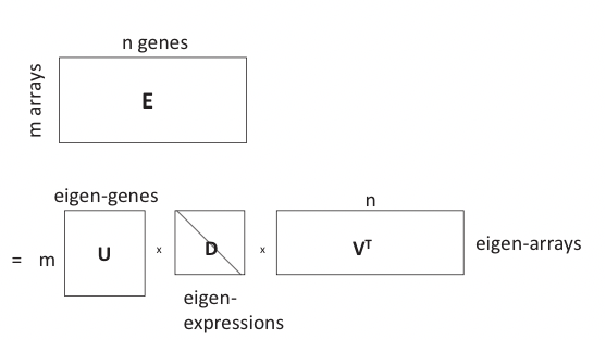
When analyzing microarray-based gene expression data, we are often dealing with data matrices of dimensions \(m \times n\) where m is the number of arrays and n is the number of genes. Usually n is in the order of thousands and m is in the order of hundreds. We would like to identify the most important features (genes) that best explain the expression variation, or patterns, in the dataset. This can be done by performing PCA on the expression matrix:

\[\mathbf{E}=\mathbf{U D V}^{T} \nonumber \]

This is in essence an SVD of the expression matrix E that rotates and scales the feature space so that expression vectors of each gene in the new orthogonal coordinate system are as uncorrelated as possible, where E is the m by n expression matrix, U is the m by m matrix of left singular vectors (i.e. principal components), or “eigen-genes”, V is the n by n matrix of right singular vectors, or “eigen-arrays”, and D is a diagonal matrix of singular values, or “eigen-expressions” of eigen-genes. This is illustrated in Figure 20.6.

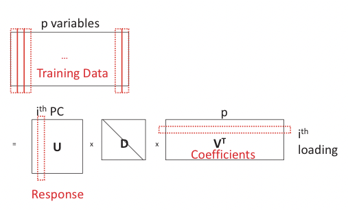
In PCA, each principal component (eigen-gene, a column of U) is a linear combination of n variables (genes), which corresponds to a loading vector (column of V) where the loadings are coecients corresponding to variables in the linear combination.

However, a straightforward application of PCA to expression matrices or any large data matrices can be problematic because the principal components (eigen-genes) are linear combinations of all n variables (genes), which is difficult to interpret in terms of functional relevance. In practice we would like to use a combination of as few genes as possible to explain expression patterns, which can be achieved by a sparse version of PCA.

source unknown. All rights reserved. This content is excluded from our Creative Commons license. For more information, see http://ocw.mit.edu/help/faq-fair-use/.

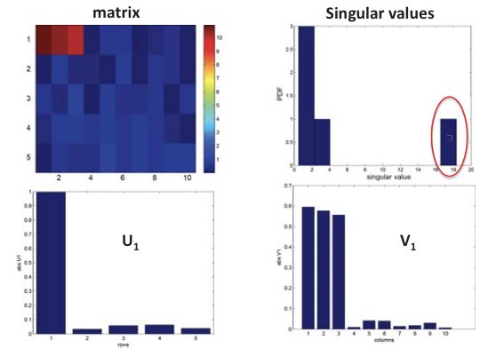
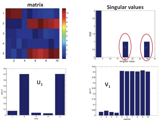
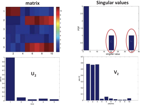
Figure 20.5: Structural inference using SVD

Sparse PCA

Sparse PCA (SPCA) modifies PCA to constrain the principal components (PCs) to have sparse loadings, thus reducing the number of explicitly used variables (genes in microarray data, etc.) and facilitating interpretation. This is done by formulating PCA as a linear regression-type optimization problem and imposing sparsity constraints.

A linear regression problem takes a set of input variables x = (1,x₁,...,x_p) and response variables \(\mathbf{y}=\mathbf{x} \beta+\epsilon\) where \(\beta\) is a row vector of regression coefficients \(\left(\beta_{0}, \beta_{1}, \ldots, \beta_{p}\right)^{T}\) and \(\epsilon\) is the error. The regression model for N observations can be written in matrix form:

\[\left[\begin{array}{c}
y_{1} \\
y_{2} \\
\vdots \\
y_{N}
\end{array}\right]=\left[\begin{array}{ccccc}
1 & x_{1,1} & x_{1,2} & \cdots & x_{1, p} \\
1 & x_{2,1} & x_{2,2} & \cdots & x_{2, p} \\
\vdots & \vdots & \vdots & \ddots & \vdots \\
1 & x_{N, 1} & x_{N, 2} & \cdots & x_{N, p}
\end{array}\right]\left[\begin{array}{c}
\beta_{0} \\
\beta_{1} \\
\vdots \\
\beta_{p}
\end{array}\right]+\left[\begin{array}{c}
\epsilon_{1} \\
\epsilon_{2} \\
\vdots \\
\epsilon_{N}
\end{array}\right] \]

The goal of the linear regression problem is to estimate the coefficients \(\beta\). There are several ways to do this, and the most commonly used methods include the least squares method, the Lasso method and the elastic net method.

Least Squares method minimizes the residual sum of squared error:

Figure 20.6: Eigen-gene decomposition using PCA

\[\hat{\beta}=\operatorname{argmin}_{\beta}\{R S S(\beta) \mid D\} \]

where \(R S S\left(\beta \equiv \sum_{i=1}^{N}\left(y_{i}-X_{i} \beta\right)^{2}\right.\) (X_i is the ith instance of input variables x). This is illustrated in Figure 20.7 for the 2-D and 3-D cases, where either a regression line or hyperplane is produced.

source unknown. All rights reserved. This content is excluded from our Creative Commons license. For more information, see http://ocw.mit.edu/help/faq-fair-use/.

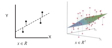
Figure 20.7: Least squares solution of linear regression. Left: 2-D case, right: 3-D case

Lasso method not only minimizes the sum of residual errors but at the same time minimizes a Lasso penalty, which is proportional to the L-1 norm of the coffiecient vector \(\beta\):

\[\hat{\beta}=\operatorname{argmin}_{\beta}\left\{R S S(\beta)+L_{1}(\beta) \mid D\right\} \]

where \(L_{1}(\beta)=\lambda \sum_{j=1}^{p}\left|\beta_{j}\right|, \lambda \geq 0\) The ideal penalty for Sparse PCA is the L₀ norm which penalizes j=1 each non-zero element by 1, while zero elements are penalized by 0. However, the L₀ penalty function is non-convex and the best solution for exploring the exponential space (number of possible combinations of non-zero elements) is NP-hard. The L₁ norm provides a convex approximation to the L₀ norm. The Lasso regression model in essence continuously shrinks the coecients toward zero as much as possible, producing a sparse model. It automatically selects for the smallest set of variables that explain variations in the data. However, the Lasso method su↵ers from the problem that if there exists a group of highly correlated variables it tends to select only one of these variables. In addition, Lasso selects at most N variables, i.e. the number of selected variables is limited by sample size.

Elastic Net method removes the group selection limitation of the Lasso method by adding a ridge constraint:

\[\hat{\beta}=\operatorname{argmin}_{\beta}\left\{R S S(\beta)+L_{1}(\beta)+L_{2}(\beta) \mid D\right\}\]

where \(L_{2}(\beta)=\lambda_{2} \sum_{j=1}^{p}\left|\beta_{j}\right|^{2}, \quad \lambda_{2} \geq 0\). In the elastic net solution, a group of highly correlated variables will be selected once one of them is included.

All of the added penalty terms above arise from the theoretical framework of regularization. We skip the mathematics behind the technique and point to an online concise explanation and tutorial of regularization at http://scikit-learn.org/stable/modul...ear_model.html.

PCA can be reconstructed in a regression framework by viewing each PC as a linear combination of the p variables. Its loadings can thus be recovered by regressing PC on the p variables (Figure 20.8). Let \(\mathbf{x}=\mathbf{U D V}^{T} . \forall i\), denote Y_i = U_iD_ii, then Y_i is the ith principal component of X. We state without proving the following theorem that confirms the correctness of reconstruction:

Theorem 20.4.1. \(\forall \lambda>0\), \(\text {suppose } \hat{\beta}_{\text {ridge}}\) is the ridge estimate given by

\[\hat{\beta}_{\text {ridge}}=\operatorname{argmin}_{\beta}\left|Y_{i}-X_{i} \beta\right|^{2}+\lambda|\beta|^{2}\nonumber\]

\[\text {and let } \hat{\mathbf{v}}=\frac{\hat{\beta}_{\text {ridge}}}{\left|\beta_{\text {ridge}}\right|}, \text {then } \hat{\mathbf{v}}=V_{i} \nonumber \]

Figure 20.8: PCA in a regression framework

Note that the ridge penalty does not penalize the coecients but rather ensure the reconstruction of the PCs. Such a regression problem cannot serve as an alternative to naive PCA as it uses exactly its results U in the model, but it can be modified by adding the Lasso penalty to the regression problem to penalize for the absolute values of coefficients:

\[\hat{\beta}_{\text {ridge}}=\operatorname{argmin}_{\beta}\left|Y_{i}-X_{i} \beta\right|^{2}+\lambda|\beta|^{2}+\lambda_{1}|\beta| \]

where \(\mathbf{X}=\mathbf{U D V}^{T}\) and \(\forall i, Y_{i}=U_{i} D_{i i}\) is the ith principal component of X. The resulting \(\hat{\beta}\) when scaled by its norm are exactly what SPCA aims at - sparse loadings:

\[\hat{V}_{i}=\frac{\hat{\beta}}{|\hat{\beta}|} \approx V_{i}\]
with \(X \hat{V}_{i} \approx Y_{i}\) being the ith sparse principal component.

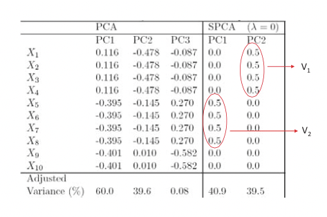
Here we give a simulated example dataset and compare the recovery of hidden factors using PCA and SPCA. We have 10 variables for which to generate data points: X = (X₁, ..., X₁₀), and a model of 3 hidden factors V₁, V₂ and V₃ is used to generate the data:

\[\begin{array}{l}
V_{1} \sim N(0,290) \\
V_{2} \sim N(0,300) \\
V_{3} \sim-0.3 V_{1}+0.925 V_{2}+e, e \sim N(0,1) \\
X_{i}=V_{1}+e_{i}^{1}, e_{i}^{1} \sim N(0,1), i=1,2,3,4 \\
X_{i}=V_{2}+e_{i}^{2}, e_{i}^{2} \sim N(0,1), i=5,6,7,8 \\
X_{i}=V_{3}+e_{i}^{3}, e_{i}^{3} \sim N(0,1), i=9,10
\end{array}\nonumber \]

From these data we expect two significant structures to arise from a sparse PCA model, each governed by hidden factors V₁ and V₂ respectively (V₃ is merely a linear mixture of the two). Indeed, as shown in Figure 20.9, by limiting the number of variables used, SPCA correctly recovers the PCs explaining the effects of V₁ and V₂ while PCA does not distinguish well among the mixture of hidden factors.

Figure 20.9: PCA vs SPCA