20.3: Linear Algebra Review

Last updated
Save as PDF

Page ID: 41037

\( \newcommand{\vecs}[1]{\overset { \scriptstyle \rightharpoonup} {\mathbf{#1}} } \) \( \newcommand{\vecd}[1]{\overset{-\!-\!\rightharpoonup}{\vphantom{a}\smash {#1}}} \)\(\newcommand{\id}{\mathrm{id}}\) \( \newcommand{\Span}{\mathrm{span}}\) \( \newcommand{\kernel}{\mathrm{null}\,}\) \( \newcommand{\range}{\mathrm{range}\,}\) \( \newcommand{\RealPart}{\mathrm{Re}}\) \( \newcommand{\ImaginaryPart}{\mathrm{Im}}\) \( \newcommand{\Argument}{\mathrm{Arg}}\) \( \newcommand{\norm}[1]{\| #1 \|}\) \( \newcommand{\inner}[2]{\langle #1, #2 \rangle}\) \( \newcommand{\Span}{\mathrm{span}}\) \(\newcommand{\id}{\mathrm{id}}\) \( \newcommand{\Span}{\mathrm{span}}\) \( \newcommand{\kernel}{\mathrm{null}\,}\) \( \newcommand{\range}{\mathrm{range}\,}\) \( \newcommand{\RealPart}{\mathrm{Re}}\) \( \newcommand{\ImaginaryPart}{\mathrm{Im}}\) \( \newcommand{\Argument}{\mathrm{Arg}}\) \( \newcommand{\norm}[1]{\| #1 \|}\) \( \newcommand{\inner}[2]{\langle #1, #2 \rangle}\) \( \newcommand{\Span}{\mathrm{span}}\)\(\newcommand{\AA}{\unicode[.8,0]{x212B}}\)

Our goal of this section is to remind you of some concepts you learned in your linear algebra class. This is not meant to be a detailed walk through. If you would want to learn more about any of the following concepts, I recommend picking up a linear algebra book and reading from that section. But this will serve as a good reminder and noting concepts that are important for us in this chapter.

Eigenvectors

Given a square matrix A, \((m \times m)\), the eigenvector v is the solution to the following equation.

\[A v=\lambda v \nonumber \]

In other words, if we multiply the matrix by that vector, we only change our position parallel the vector (we get back a scaled version of the vector v).

And \(\lambda\) (how much the vector v is scaled) is called the eigenvalue.
So how many eigenvalues are there at most? Let’s take the first steps to solving this equation.

\[A v=\lambda v \Rightarrow(A-\lambda I) v=0 \nonumber \]
that has non-zero solutions when \(|A-\lambda I|=0\). That is an m-th order equation in \(\lambda\) which can have at most m distinct solutions. Remember that those solutions can be complex, even though A is real.

Vector decomposition

Since the eigenvectors form the set of all bases they fully represent the column space. Given that, we can decompose any arbitrary vector x to a combination of eigenvectors.

\[x=\sum_{i} c_{i} v_{i} \nonumber \]

Thus when we multiply a vector with a matrix A, we can rewrite it in terms of the eigenvectors.

\[\begin{array}{c}
A x=A\left(c_{1} v_{1}+c_{2} v_{2}+\ldots\right) \\
A x=c_{1} A v_{1}+c_{2} A_{v} 2+\ldots \\
A x=c_{1} \lambda_{1} v_{1}+c_{2} \lambda_{2} v_{2}+c_{3} \lambda_{3} v_{3}+\ldots
\end{array} \nonumber \]
So the action of A on x is determined by the eigenvalues of and eigenvectors. And we can observe that small eigenvalues have a small e↵ect on the multiplication.

Did You Know?

• For symmetric matrices, eigenvectors for distinct eigenvalues are orthogonal.

• All eigenvalues of a real symmetric matrix are real.
• All eigenvalues of a positive semidefinite matrix are non-negative.

Diagonal Decomposition

Also known as Eigen Decomposition. Let S be a square \(m \times m \) matrix with m linearly independent eigenvectors (a non-defective matrix).

Then, there exist a decomposition (matrix digitalization theorem) \[ S=U \Lambda U^{-1} \nonumber \]

Where the columns of U are the eigenvectors of S. And \(\Lambda\) is a diagonal matrix with eigenvalues in its diagonal.

Singular Value Decomposition

Oftentimes, singular value decomposition (SVD) is used for the more general case of factorizing an \(m \times n\) non-square matrix:

\[\mathbf{A}=\mathbf{U} \boldsymbol{\Sigma} \mathbf{V}^{T}\]

where U is a \(m \times m \) matrix representing orthogonal eigenvectors of AA^_T , V is a \(n \times n \) matrix representing orthogonal eigenvectors of A^TA and V is a \(n \times n\) matrix representing square roots of the eigenvalues of A^T A (called singular values of A):

\[ \mathbf{\Sigma}=\operatorname{diag}\left(\sigma_{1}, \ldots, \sigma_{r}\right), \sigma_{i}=\sqrt{\lambda_{i}} \]

The SVD of any given matrix can be calculated with a single command in Matlab and we will not cover the technical details of computing it. Note that the resulting “diagonal” matrix \(\mathbf{\Sigma} \) may not be full-rank, i.e. it may have zero diagonals, and the maximum number of non-zero singular values is min(m, n).

For example, let

\[A=\left[\begin{array}{cc}
1 & -1 \\
1 & 0 \\
1 & 0
\end{array}\right] \nonumber \]

thus m=3, n=2. Its SVD is

\[\left[\begin{array}{ccc}
0 & \frac{2}{\sqrt{6}} & \frac{1}{\sqrt{3}} \\
\frac{1}{\sqrt{2}} & -\frac{1}{\sqrt{6}} & \frac{1}{\sqrt{3}} \\
\frac{1}{\sqrt{2}} & \frac{1}{\sqrt{6}} & -\frac{1}{\sqrt{3}}
\end{array}\right]\left[\begin{array}{cc}
1 & 0 \\
0 & \sqrt{3} \\
0 & 0
\end{array}\right]\left[\begin{array}{cc}
\frac{1}{\sqrt{2}} & \frac{1}{\sqrt{2}} \\
\frac{1}{\sqrt{2}} & -\frac{1}{\sqrt{2}}
\end{array}\right] \nonumber \]

Typically, the singular values are arranged in decreasing order.

SVD is widely utilized in statistical, numerical analysis and image processing techniques. A typical application of SVD is optimal low-rank approximation of a matrix. For example if we have a large matrix of data ,e.g. 1000 by 500, and we would like to approximate it with a lower-rank matrix without much loss of information, formulated as the following optimization problem:

Find A_k of rank k such that \(\mathbf{A}_{k}=\min _{\mathbf{X}: r a n k(\mathbf{X})=k}\|\mathbf{A}-\mathbf{X}\|_{F} \)

where the subscript F denotes Frobenius norm \(\|\mathbf{A}\|_{F}=\sqrt{\sum_{i} \sum_{j}\left|a_{i j}\right|^{2}}\). Usually k is much smaller than r. The solution to this problem is the SVD of X, \(\mathbf{U} \boldsymbol{\Sigma} \mathbf{V}^{T}\), with the smallest r-k singular values in \(\mathbf{\Sigma}\) set to zero:

\[\mathbf{A}_{k}=\operatorname{Udiag}\left(\sigma_{1}, \ldots, \sigma_{k}, \ldots, 0\right) \mathbf{V}^{T} \nonumber \]

Such an approximation can be shown to have an error of \(\left\|\mathbf{A}-\mathbf{A}_{k}\right\|_{F}=\sigma_{k+1}\). This is also known as the Eckart-Young theorem.

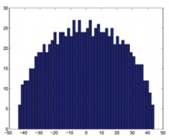
A common application of SVD to network analysis is using the distribution of singular values of the adjacency matrix to assess whether our network looks like a random matrix. Because the distribution of the singular values (Wigner semicircle law) and that of the largest eigenvalue of a matrix (Tracy-Widom distribution) have been theoretically derived, it is possible to derive the distribution of eigenvalues (singular values in SVD) of an observed network (matrix), and calculate a p-value for each of the eigenvalues. Then we need only look at the significant eigenvalues (singular values) and their corresponding eigenvectors (singular vectors) to examine significant structures in the network. The following figure shows the distribution of singular values of a random Gaussian unitary ensemble (GUE, see this Wikipedia link for definition and properties en.Wikipedia.org/wiki/Random_matrix) matrix, which form a semi-circle according to Wigner semicircle law (Figure 20.4).

An example of using SVD to infer structural patterns in a matrix or network is shown in Figure 20.5. The top-left panel shows a structure (red) added to a random matrix (blue background in the heatmap), spanning the first row and first three columns. SVD detects this by the identification of a large singular value (circled in red on singular value distribution) and corresponding large row loadings (U1) as well as three large column loadings (V1). As more structures are added to the network (top-right and bottom panels), they can be discovered using SVD by looking at the next largest singular values and corresponding row/column loadings, etc..