20.2: Network Centrality Measures

We discussed in the previous chapter how we can take a biological network and model it mathematically. Now as we visualize these graphs and try to understand them we need some measure for the importance of a node/edge to the structural characteristics of the system. There are many ways to measure the importance (what we refer to as centrality) of a node. In this chapter we will explore these ideas and investigate their significance.

Degree Centrality

The first idea about centrality is measure importance by the degree of a node. This is probably one of the most intuitive centrality measures as it’s very easy to visualize and reason about. The more edges you have connected to you, the more important to the network you are.

Let’s explore a simple example and see how the go about finding these centralities. We have the following graph

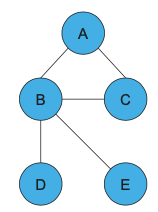
And our goal is to find the degree centrality of every node in the graph. To proceed, we first write out the adjacency matrix for this graph. The order for the edges is A, B, C, D, E

\[A=\left[\begin{array}{lllll}
0 & 1 & 1 & 0 & 0 \\
1 & 0 & 1 & 1 & 1 \\
1 & 1 & 0 & 0 & 0 \\
0 & 1 & 0 & 0 & 0 \\
0 & 1 & 0 & 0 & 0
\end{array}\right]\]

Previously we discussed how to find the degree for a node given an adjacency matrix. We sum along every row of the adjacency matrix.

\[D=\left[\begin{array}{l}
1 \\
4 \\
3 \\
1 \\
1
\end{array}\right]\]

Now D is a vector with the degree of every node. This vector gives us a relative centrality measures for nodes in this network. We can observe that node B has the highest degree centrality.

Although this metric gives us a lot of insight, it has its limitations. Imagine a situation where there is one node that connects two parts of the network together. The node will have a degree of 2, but it is much more important than that.

Betweenness Centrality

Betweenness centrality gives us another way to think about importance in a network. It measures the number of shortest paths in the graph that pass through the node divided by the total number of shortest paths. In other words, this metric computes all the shortest paths between every pair of nodes and sees what is the percentage of that passes through node k. That percentage gives us the centrality for node k.

• Nodes with high betweenness centrality control information flow in a network.

• Edge betweenness is defined in a similar fashion.

Closeness Centrality

In order to properly define closeness we need to define the term farness. Distance between two nodes is the shortest paths between them. The farness of a node is the sum of distances between that node and all other nodes. And the closeness of a node is the inverse of its farness. In other words, it is the normalized inverse of the sum of topological distances in the graph.

The most central node is the node that propagates information the fastest through the network.

The description of closeness centrality makes it similar to the degree centrality. Is the highest degree centrality always the highest closeness centrality? No. Think of the example where one node connects two components, that node has a low degree centrality but a high closeness centrality.

Eigenvector Centrality

The eigenvector centrality extends the concept of a degree. The best to think of it is the average of the centralities of it’s network neighbors. The vector of centralities can be written as:

\[x=\frac{1}{\lambda} A x \nonumber \]
where A is the adjacency matrix. The solution to the above equation is going to be the eigenvector corresponding to the principle component (largest eigenvalue).
The following section includes a review of linear algebra concepts including eigenvalue and eigenvectors.