
20.1: Introduction
- Page ID
- 41035

Molecular and cellular biology describe a hugely diverse system of interacting components that is capable of producing intricate and complex phenomena. Interactions within the proteome describe cellular metabolism, signaling cascades, and response to the environment. Networks are a valuable tool to assist in representing, understanding, and analyzing the complex interactions between biological components. Living systems can be viewed as a composition of multiple layers that each encode information about the system. Some important layers are:
- Genome: Includes coding and non-coding DNA. Genes defined by coding DNA are used to build RNA, and Cis-regulatory elements regulate the expression of these genes.
- Epigenome: Defined by chromatin configuration. The structure of chromatin is based on the way that histones organize DNA. DNA is divided into nucleosome and nucleosome-free regions, forming its final shape and influencing gene expression.1
- Transcriptome RNAs (ex. mRNA, miRNA, ncRNA, piRNA) are transcribed from DNA. They have regulatory functions and manufacture proteins.
- Proteome Composed of proteins. This includes transcription factors, signaling proteins, and metabolic enzymes.
Each layer consists of a network of interactions. For example, mRNAs and miRNAs interact to regulate the production of proteins. Layers can also interact with each other, forming a network between networks. For example, a long non-coding RNA called Xist produces epigenomic changes on the X-chromosome to achieve dosage compensation through X-inactivation.
Introducing Biological Networks
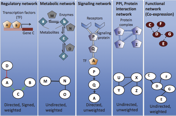
Five example types of biological networks:
Regulatory Network – set of regulatory interactions in an organism.
• Nodes represent regulators (ex. transcription factors) and associated targets.
• Edges represent regulatory interaction, directed from the regulatory factor to its target. They are signed according to the positive or negative e↵ect and weighted according to the strength of the reaction.
Metabolic Network – connects metabolic processes. There is some flexibility in the representation, but an example is a graph displaying shared metabolic products between enzymes.
• Nodes represent enzymes.
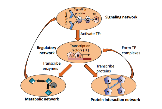
Figure 20.1: Interactions between biological networks.
• Edges represent regulatory reactions, and are weighted according to the strength of the reaction. Edges are undirected.
Signaling Network – represents paths of biological signals.
- Nodes represent proteins called signaling receptors.
- Edges represent transmitted and received biological signals, directed from transmitter to receiver. Edges are directed and unweighted.
Protein Network – displays physical interactions between proteins.
- Nodes represent individual proteins.
- Edges represent physical interactions between pairs of proteins. These edges are undirected and unweighted.
Coexpression Network – describes co-expression functions between genes. Quite general; represents functional rather than physical interaction networks, unlike the other types of nets. Powerful tool in computational analysis of biological data.
• Nodes represent individual genes.
• Edges represent co-expression relationships. These edges are undirected and unweighted.
Today, we will focus exclusively on regulatory networks. Regulatory networks control context-specific gene expression, and thus have a great deal of control over development. They are worth studying because they are prone to malfunction and are associated with disease.
Interactions Between Biological Networks
Individual biological networks (that is, layers) can themselves be considered nodes in a larger network repre- senting the entire biological system. We can, for example, have a signaling network sensing the environment governing the expression of transcription factors. In this example, the network would display that TFs govern the expression of proteins, proteins can play roles as enzymes in metabolic pathways, and so on.
The general paths of information exchange between these networks are shown in figure 21.1a.
source unknown. All rights reserved. This content is excluded from our Creative Commons license. For more information, see ocw.mit.edu/help/faq-fiar-use/.
Network Representation
In figure 20.2 we show a number of these networks and their visualizations as graphs. However, how did we decide on these particular networks to represent the underlying biological models? Given a large biological dataset, how can we understand dependencies between biological objects and what is the best way to model these dependencies? Below, we introduce several approaches to network representation. In practice, no model is perfect. Model choice should balance biological knowledge and computability for reasonably ecient analysis.
Networks are typically described as graphs. Graphs are composed of 1. nodes, which represent objects; and 2. edges, which represent connections or interactions between nodes. There are three main ways to think about biological networks as graphs.
Probabilistic Networks – also known as graphical models. They model a probability distribution between nodes.
- Modeling joint probability distribution of variables using graphs.
- Some examples are Bayesian Networks (directed), Markov Random Fields (Undirected). More on Bayesian networks in the later chapters.
Physical Networks – In this scheme we usually think of nodes as physically interacting with each other and the edges capture that interaction.
• Edges represent physical interaction among nodes. • Example: physical regulatory networks.
Relevance Network – Model the correlation between nodes. • Edge weights represent node similarities.
• Example: functional regulatory networks.
Networks as Graphs
Computer scientists consider subtypes of graphs, each with different properties for their edges and nodes.
• Weighted graph: Edges have an associated weight. Weights are generally positive. When all the weights are 1, then we call it an unweighted graph.
• Directed graphs: Edges possess directionality. For example A ! B is not the same as A B. When the edges do not have direction, we call it an undirected graph.
• Multigraphs (pseudographs): When we allow more than one edge to go between two nodes (more than two if it’s directed) then we call it a multigraph. This can be useful for modeling multiple interactions between two nodes each with di↵erent weights for example.
• Simple graph: All edges are undirected and unweighted. Multiple edges between nodes and self-edges are forbidden.
Matrix Representation of Graphs
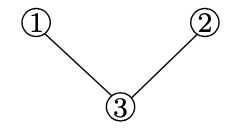
Adjacency matrix One way to represent a network is using the so-called adjacency matrix. The adjacency matrix of a network with n nodes is an \(n \times n\) matrix A where Aij is equal to one if there is an edge between nodes i and j, and 0 otherwise. For example, the adjacency matrix of the graph represented in figure 21.6b is given by:
\[ A=\left[\begin{array}{lll}
0 & 0 & 1 \\
0 & 0 & 1 \\
1 & 1 & 0
\end{array}\right] \]
If the network is weighted (i.e., if the edges of the network each have an associated weight), the definition of the adjacency matrix is modified so that Aij holds the weight of the edge between i and j if the edge exists, and zero otherwise.
Another convenience that comes with the adjacency matrix representation is that when we have a binary matrix (unweighted graph) then the sum of row i gives us the degree of node i. In an undirected graph, the degree of a node is the number of edges it has. Since every entry in the row tells us whether node i is connected to another node, by summing all these values we know how many nodes is node i connected to, thus we get the degree.
1More in the epigenetics lecture.