In this lecture, we learned how chromatin marks can be used to infer biologically relevant states. The analysis in [7] presents a sophisticated method to apply previously learned techniques such as HMMs to a complex problem. The lecture also introduced the powerful Burrows-Wheeler transform that has enabled ecient read mapping.
Bibliography
[1] Langmead B, Trapnell C, Pop M, and Salzberg S. Ultrafast, memory-ecient alignment of short DNA sequences to the human genome. Genome Biology, 10(3), 2009.
[2] Roadmap Epigenomics Consortium, Kundaje A, Meuleman W, et al. Integrative analysis of 111 reference human epigenomes. Nature, 518(7539):317–330, 2015.
[3] The ENCODE Project Consortium. An integrated encyclopedia of DNA elements in the human genome. Nature, 489(7414):57–74, 2012.
[4] Heard E and Martienssen RA. Transgenerational epigenetic inheritance: Myths and mechanisms. Cell, 157(1):95–109, 2014.
[5] Mardis ER. ChIP-seq: welcome to the new frontier. Nature Methods, 4(8):614–614, 2007.
[6] Herz H-M, Hu D, and Shilatifard A. Enhancer malfunction in cancer. Molecular Cell, 53(6):859–866, 2014.
[7] Ernst J and Kellis M. Discovery and characterization of chromatin states for systematic annotation of the human genome. Nature Biotechnology, 28:817–825, 2010.
[8] Ernst J, Kheradpour P, Mikkelsen TS, et al. Mapping and analysis of chromatin state dynamics in nine human cell types. Nature, 473(7345):43–49, 2011.
[9] Mousavi K, Zare H, Dell’orso S, Grontved L, et al. eRNAs promote transcription by establishing chromatin accessibility at defined genomic loci. Molecular Cell, 51(5):606–17, 2013.
[10] Qunhua Li, James B. Brown, Haiyan Huang, and Peter J. Bickel. Measuring reproducibility of high-throughput experiments. The Annals of Applied Statistics, 5(3):1752–1779, 2011.
[11] Li Y and Tollefsbol TO. DNA methylation detection: Bisulfite genomic sequencing analysis. Methods Molecular Biology, 791:11–21, 2011.
Courtesy of National Institutes of Health. Image in the public domain (left).
Courtesy of Elsevier, Inc. Used with permission. Source: Herz, Hans-Martin, Deqing Hu, et al. "Enhancer Malfunction in Cancer." Molecular Cell 53, no. 6 (2014): 859-66 (right).
Figure 19.1: A. There is a wide diversity of modifications in the epigenome. Some regions of DNA are compactly wound around histones, making the DNA inaccessible and the genes inactive. Other regions have more accessible DNA and thus active genes. Epigenetic factors can bind to the tails of these histones to modify these properties. B. Histone modifications provide information about what types of proteins are bound to the DNA and what the function of the region is. In this example, The histone modifications allow for an enhancer region (potentially over 100 kilo bases away) to interact with the promoter region. [6]
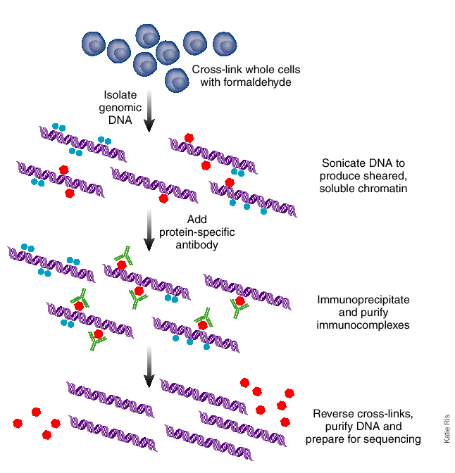
Figure 19.2: The method of chromatin immunoprecipitation [5]. The steps in this figure correspond to the six steps of the procedure.Figure 19.3: (Top) In the Burrows-Wheeler forward transformation rotations are generated and sorted. The last column of the sorted list (bolded) consists of the transformed string. (Bottom)In the Burrows-Wheeler reverse transformation the transformed string is sorted, and two columns are generated: one consisting of the original string and the other consisting of the sorted. These e↵ectively form two columns from the rotations in the forward transformation. This process is repeated until the complete rotations are generated.Figure 19.4: To use input DNA as a control, one can run the ChIP experiment as normal while simultaneously running the same experiment (with same DNA) without an antibody. This generates a background signal for which we can correct.
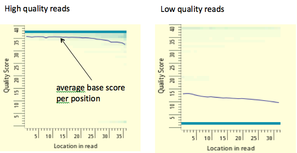
Figure 19.5: In the figure above each column is a color-coded histogram that encodes the fraction of all mapped reads that have base score Q (y-axis) at each position(x-axis). A low average per base score implies greater probability of mismappings. We typically reject reads whose average score Q is less than 10.source unknown. All rights reserved. This content is excluded from our Creative Commons license. For more information, see http://ocw.mit.edu/help/faq-fair-use/.
Figure 19.6: A sample signal track. Here, the red signal is derived from the number of reads that mapped to the genome at each position for a ChIP-seq experiment with the target H3K36me3. The signal gives a level of enrichment of the mark
Figure 19.7: Sample signal tracks for both the true experiment and the background (control). Regions are considered to have statistically significant enrichment when the true experiment signal values are well above the background signal values.Courtesy of Macmillan Publishers Limited. Used with permission. Source: Ernst, Jason, and Manolis Kellis. "Discovery and Characterization of Chromatin States for Systematic Annotation of the Human Genome." Nature Biotechnology 28, no. 8 (2010): 817-25.
Figure 19.8: Example of the data and the annotation from the HMM model. The bottom section shows the raw number of reads mapped to the genome. The top section shows the annotation from the HMM model.
Figure 19.9: Emission probabilities for the final model with 51 states. The cell corresponding to mark i and state k represents the probability that mark i is observed in state k.Figure 19.10: Transition probabilities for the final model with 51 states. The transition probability increases from green to red. Spatial relationships between neighboring chromatin states and distinct sub-groups of states are revealed by clustering the transition matrix. Notably, the matrix is sparse, so indicating that most are not possible.Figure 19.11: Chromatin state definition and functional interpretation. [7] a. Chromatin mark combinations associated with each state. Each row shows the specific combination of marks associated with each chromatin state and the frequencies between 0 and 1 with which they occur in color scale. These correspond to the emission probability parameters of the HMM learned across the genome during model training. b. Genomic and functional enrichments of chromatin states, including fold enrichment in di↵erent part of the genome (e.g. transcribed regions, TSS, RefSeq 5 end or 3end of the gene etc), in addition to fold enrichment for evolutionarily conserved elements, DNaseI hypersensitive sites, CpG islands, etc. All enrichments are based on the posterior probability assignments. c. Brief description of biological state function and interpretation (chr, chromatin; enh, enhancer).