
5.3: Genome Assembly II- String graph methods
- Page ID
- 40937

Shotgun sequencing, which is a more modern and economic method of sequencing, gives reads that around 100 bases in length. The shorter length of the reads results in a lot more repeats of length greater than that of the reads. Hence, we need new and more sophisticated algorithms to do genome assembly correctly.
String graph definition and construction
The idea behind string graph assembly is similar to the graph of reads we saw in section 5.2.2. In short, we are constructing a graph in which the nodes are sequence data and the edges are overlap, and then trying to find the most robust path through all the edges to represent our underlying sequence.
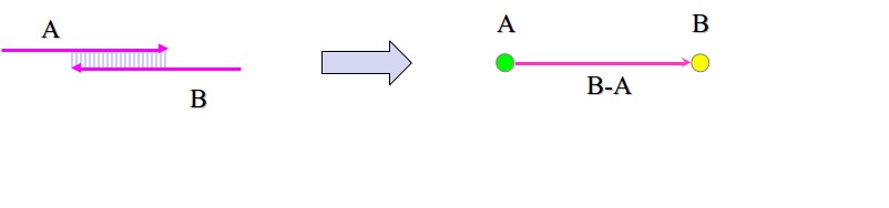
Figure 5.10: Constructing a string graph.
Starting from the reads we get from Shotgun sequencing, a string graph is constructed by adding an edge for every pair of overlapping reads. Note that the vertices of the graph denote junctions, and the edges correspond to the string of bases. A single node corresponds to each read, and reaching that node while traversing the graph is equivalent to reading all the bases upto the end of the read corresponding to the node. For example, in figure 5.10, we have two overlapping reads A and B and they are the only reads we have. The corresponding string graph has two nodes and two edges. One edge doesn’t have a vertex at its tail end, and has A at its head end. This edge denotes all the bases in read A. The second edge goes from node A to node B, and only denotes the bases in B-A (the part of read B which is not overlapping with A). This way, when we traverse the edges once, we read the entire region exactly once. In particular, notice that we do not traverse the overlap of read A and read B twice.
© source unknown. All rights reserved. This content is excluded from our Creative Commons license. For more information, see http://ocw.mit.edu/help/faq-fair-use/.
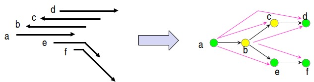
Figure 5.11: Constructing a string graph 99
There are a couple of subtleties in the string graph (figure 5.11) which need mentioning:
- We have two different colors for nodes since the DNA can be read in two directions. If the overlap is between the reads as is, then the nodes receive same colors. And if the overlap is between a read and the complementary bases of the other read, then they receive different colors.
- Secondly, if A and B overlap, then there is ambiguity in whether we draw an edge from A to B, or from B to A. Such ambuigity needs to be resolved in a consistent manner at junctions caused due to repeats.
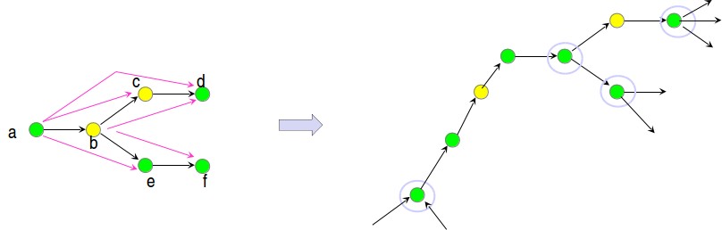
Figure 5.12: Example of string graph undergoing removal of transitive edges.
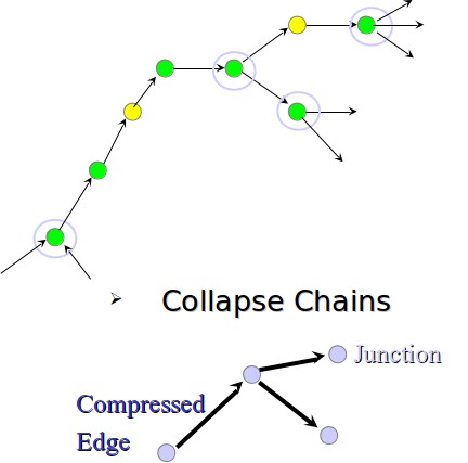
Figure 5.13: Example of string graph undergoing chain collapsing.
After constructing the string graph from overlapping reads, we:-
• Remove transitive edges: Transitive edges are caused by transitive overlaps, i.e. A overlap B overlaps C in such a way that A overlaps C. There are randomized algorithms which remove transitive edges in O(E) expected runtime. In figure 5.12, you can see the an example of removing transitive edges.
• Collapse chains: After removing the transitive edges, the graph we build will have many chains where each node has one incoming edge and one outgoing edge. We collapse all these chains to a single edge. An example of this is shown in figure 5.13.
Flows and graph consistency
After doing everything mentioned above we will get a pretty complex graph, i.e. it will still have a number of junctions due to relatively long repeats in the genome compared to the length of the reads. We will now see how the concepts of flows can be used to deal with repeats.
First, we estimate the weight of each edge by the number of reads we get corresponds to the edge. If we have double the number of reads for some edge than the number of DNAs we sequenced, then it is fair to assume that this region of the genome gets repeated. However, this technique by itself is not accurate enough. Hence sometimes we may make estimates by saying that the weight of some edge is ≥ 2, and not assign a particular number to it.
Figure 5.14: Left: Flow resolution concept. Right: Flow resolution example
We use reasoning from flows in order to resolve such ambiguities. We need to satisfy the flow constraint at every junction, i.e. the total weight of all the incoming edges must equal the total weight of all the outgoing edges. For example, in the figure 5.14 there is a junction with an incoming edge of weight 1, and two outgoing edges of weight ≥ 0 and ≥ 1. Hence, we can infer that the weights of the outgoing edges are exactly equal to 0 and 1 respectively. A lot of weights can be inferred this way by iteratively applying this same process throughout the entire graph.
Feasible flow
Once we have the graph and the edge weights, we run a min cost flow algorithm on the graph. Since larger genomes may not a have unique min cost flow, we iteratively do the following:
• Add ε penalty to all edges in solution
• Solve flow again - if there is an alternate min cost flow it will now have a smaller cost relative to the previous flow
• Repeat until we find no new edges
After doing the above, we will be able to label each edge as one of the following
• Required: edges that were part of all the solutions
• Unreliable: edges that were part of some of the solutions
• Not required: edges that were not part of any solution
Dealing with sequencing errors
There are various sources of errors in the genome sequencing procedure. Errors are generally of two different kinds, local and global.
Local errors include insertions, deletions and mutations. Such local errors are dealt with when we are looking for overlapping reads. That is, while checking whether reads overlap, we check for overlaps while being tolerant towards sequencing errors. Once we have computed overlaps, we can derive a consensus by mechanisms such as removing indels and mutations that are not supported by any other read and are contradicted by at least 2.
Global errors are caused by other mechasisms such as two different sequences combining together before being read, and hence we get a read which is from different places in the genome. Such reads are called chimers. These errors are resolved while looking for a feasible flow in the network. When the edge corresponding to the chimer is in use, the amount of flow going through this edge is smaller compared to the flow capacity. Hence, the edge can be detected and then ignored.
Each step of the algorithm is made as robust and resilient to sequencing errors as possible. And the number of DNAs split and sequenced is decided in a way so that we are able to construct most of the DNA (i.e. fulfill some quality assurance such as 98% or 95%).
Resources
Some popular genome assemblers using String Graphs are listed below
- Euler (Pevzner, 2001/06) : Indexing → deBruijn graphs → picking paths → consensus
- Valvel (Birney, 2010) : Short reads → small genomes → simplification → error correction
- ALLPATHS (Gnerre, 2011) : Short reads → large genomes → jumping data → uncertainty