1.5: Introduction to algorithms and probabilistic inference

Last updated
Save as PDF

Page ID: 40910

\( \newcommand{\vecs}[1]{\overset { \scriptstyle \rightharpoonup} {\mathbf{#1}} } \) \( \newcommand{\vecd}[1]{\overset{-\!-\!\rightharpoonup}{\vphantom{a}\smash {#1}}} \)\(\newcommand{\id}{\mathrm{id}}\) \( \newcommand{\Span}{\mathrm{span}}\) \( \newcommand{\kernel}{\mathrm{null}\,}\) \( \newcommand{\range}{\mathrm{range}\,}\) \( \newcommand{\RealPart}{\mathrm{Re}}\) \( \newcommand{\ImaginaryPart}{\mathrm{Im}}\) \( \newcommand{\Argument}{\mathrm{Arg}}\) \( \newcommand{\norm}[1]{\| #1 \|}\) \( \newcommand{\inner}[2]{\langle #1, #2 \rangle}\) \( \newcommand{\Span}{\mathrm{span}}\) \(\newcommand{\id}{\mathrm{id}}\) \( \newcommand{\Span}{\mathrm{span}}\) \( \newcommand{\kernel}{\mathrm{null}\,}\) \( \newcommand{\range}{\mathrm{range}\,}\) \( \newcommand{\RealPart}{\mathrm{Re}}\) \( \newcommand{\ImaginaryPart}{\mathrm{Im}}\) \( \newcommand{\Argument}{\mathrm{Arg}}\) \( \newcommand{\norm}[1]{\| #1 \|}\) \( \newcommand{\inner}[2]{\langle #1, #2 \rangle}\) \( \newcommand{\Span}{\mathrm{span}}\)\(\newcommand{\AA}{\unicode[.8,0]{x212B}}\)

1. We will quickly review some basic probability by considering an alternate way to represent motifs: a position weight matrix (PWM). We would like to model the fact that proteins may bind to motifs that are not fully specified. That is, some positions may require a certain nucleotide (e.g. A), while others positions are free to be a subset of the 4 nucleotides (e.g. A or C). A PWM represents the set of all DNA sequences that belong to the motif by using a matrix that stores the probability of finding each of the 4 nucleotides in each position in the motif. For example, consider the following PWM for a motif with length 4:

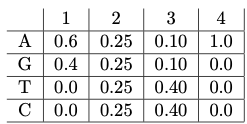
Screen_Shot_2020-07-11_at_6.54.25_PM.png

We say that this motif can generate sequences of length 4. PWMs typically assume that the distribution of one position is not influenced by the base of another position. Notice that each position is associated with a probability distribution over the nucleotides (they sum to 1 and are nonnegative).

2. We can also model the background distribution of nucleotides( the distribution found across the genome):

Screen Shot 2020-07-11 at 6.56.38 PM.png

Notice how the probabilities for A and T are the same and the probabilities of G and C are the same. This is a consequence of the complementarity DNA which ensures that the overall composition of A and T, G and C is the same overall in the genome.

3. Consider the sequence \(S = GCAA.\)

The probability of the motif generating this sequence is \[P(S|M) = 0.4 × 0.25 × 0.1 × 1.0 = 0.01. \nonumber\]
The probability of the background generating this sequence \[P (S|B) = 0.4 × 0.4 × 0.1 × 0.1 = 0.0016. \nonumber\]

4. Alone this isn’t particularly interesting. However, given fraction of sequences that are generated by the motif, e.g. P(M) = 0.1, and assuming all other sequences are generated by the background (P(B) = 0.9) we can compute the probability that the motif generated the sequence using Bayes’ Rule:

\[\begin{align*} P(M|S) &= \frac{P(S|M)P(M)}{P(S)} \\[4pt] &= \frac{P(S|M)P(M)}{P(S|B)P(B)+P(S|M)P(M)} \\[4pt] &= \frac{0.01 \times 0.1}{0.0016 \times 0.9 + 0.01 \times 0.1} = 0.40984 \end{align*}\]